This post is the first part of a double post about SVMs. This part tries to help to clarify how SVMs work in theory (with 2 full developed examples). The second part (not published yet) will explain the algorithm to solve this problem using a computer: Quadratic Programming and SMO.
Index
- Basic definition of SVMs for binary classification
- Mathematical explanation
- Kernel trick
- Example 1: 2 points in a plane
- Example 2: 3 points in a plane
- Appendix A: Scalar Projection of Vectors (1 example)
- Appendix B: Lagrange Multipliers (3 examples)
Basic definition
Support vector machines (SVMs from now on) are supervised learning models used for classification and regression. The basic idea of SVMs in binary classification is to find the farthest boundary from each class.
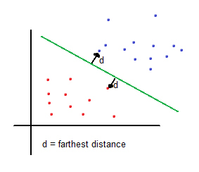
Therefore, solving a basic mathematical function given the coordinates (features) of each sample will tell whether the sample belongs to one region (class) or other. Input features determine the dimension of the problem. To keep it simple, the explanation will include examples in 2 dimensions.
Mathematical explanation
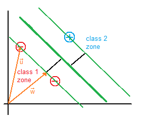
The vector  is a perpendicular vector to the boundary, but since boundary’s coefficients are unknown, vector’s coefficients are unknown as well. What we want to do is to calculate the boundary’s coefficients with respect to is a perpendicular vector to the boundary, but since boundary’s coefficients are unknown, vector’s coefficients are unknown as well. What we want to do is to calculate the boundary’s coefficients with respect to  because we have its coordinates (sample’s coordinates). because we have its coordinates (sample’s coordinates). |
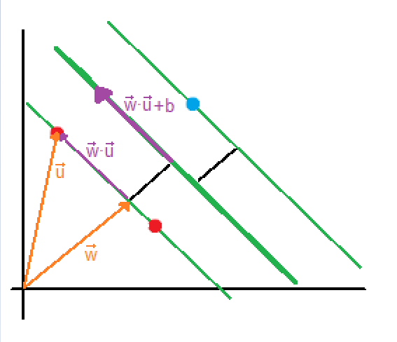
If both vectors are multiplied, the result will be the purple vector. |
Let us say that:
Where 

A new variable is now introduced:


Multiply each of them by the previous equations:

The result is the same equation. Therefore, we only need the previous formula:

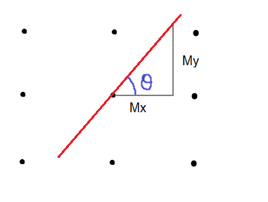
Finally, we add an additional constrain  so that the values that fulfill this, fall in between the two regions as depicted (green zone). so that the values that fulfill this, fall in between the two regions as depicted (green zone).
|
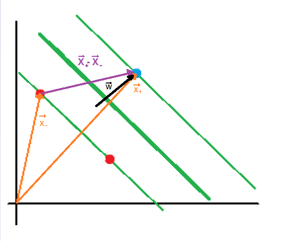
The next step is to maximize the projection of  on (the black perpendicular vector to the boundary) to keep samples from each class as far as possible. I assume that you know about scalar projection, but if you don’t, you can check out the Appendix A. on (the black perpendicular vector to the boundary) to keep samples from each class as far as possible. I assume that you know about scalar projection, but if you don’t, you can check out the Appendix A.
The length of the projection is given by the following formula: |

From the previous formula 


Therefore:

The goal is to maximize 


Thus, we have a function to minimize with a constraint (
First we have the function we want to minimize, and later the constraints.
![L = \frac{1}{2}\| w \|^2 - \sum \alpha_i [ y_i (\overrightarrow{w} \cdot \overrightarrow{x_i} +b)-1]](https://s0.wp.com/latex.php?latex=L+%3D+%5Cfrac%7B1%7D%7B2%7D%5C%7C+w+%5C%7C%5E2+-+%5Csum+%5Calpha_i+%5B+y_i+%28%5Coverrightarrow%7Bw%7D+%5Ccdot+%5Coverrightarrow%7Bx_i%7D+%2Bb%29-1%5D&bg=ffffff&fg=000&s=0&c=20201002)

Plug these two functions to 

Hence, we aim to minimize
The optimization depends on


Kernel trick
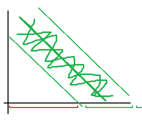
One of the most interesting properties of SVMs is that we can transform problems from a certain number of dimensions to another dimensional space. This flexibility, as known as kernel trick, allows SVMs to classify nonlinear problems.

|
 |
The following example shows how to graphically solve the XOR problem using 3 dimensions.
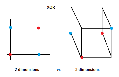
Now it is not difficult to imagine a plane that can separate between blue and red samples.
Example 1: 2 points in a plane
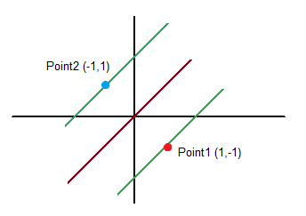
Points and class (coordinate x (x1), coordinate y (x2), class/output (y)):
![x = [-1,1]](https://s0.wp.com/latex.php?latex=x+%3D+%5B-1%2C1%5D&bg=ffffff&fg=000&s=0&c=20201002)
Class (output):

Point 2:
![x = [1,-1]](https://s0.wp.com/latex.php?latex=x+%3D+%5B1%2C-1%5D&bg=ffffff&fg=000&s=0&c=20201002)
Class (output):

We want to minimize:
We know that:
and


Let us calculate the second part of the function we want to minimize first to keep it simple:


Ergo:

Now let us calculate
![\overrightarrow{w} = \sum_{i=1}^N \alpha_i y_i x_i = \frac{1}{4} * 1 * [-1,1] + \frac{1}{4} * -1 * [1,-1] = [\frac{-1}{4} , \frac{1}{4}] + [\frac{-1}{4} , \frac{1}{4}] = [\frac{-2}{4} , \frac{2}{4}] = [\frac{-1}{2} , \frac{1}{2}]](https://s0.wp.com/latex.php?latex=%5Coverrightarrow%7Bw%7D+%3D+%5Csum_%7Bi%3D1%7D%5EN+%5Calpha_i+y_i+x_i+%3D+%5Cfrac%7B1%7D%7B4%7D+%2A+1+%2A+%5B-1%2C1%5D+%2B+%5Cfrac%7B1%7D%7B4%7D+%2A+-1+%2A+%5B1%2C-1%5D+%3D+%5B%5Cfrac%7B-1%7D%7B4%7D+%2C+%5Cfrac%7B1%7D%7B4%7D%5D+%2B+%5B%5Cfrac%7B-1%7D%7B4%7D+%2C+%5Cfrac%7B1%7D%7B4%7D%5D+%3D+%5B%5Cfrac%7B-2%7D%7B4%7D+%2C+%5Cfrac%7B2%7D%7B4%7D%5D+%3D+%5B%5Cfrac%7B-1%7D%7B2%7D+%2C+%5Cfrac%7B1%7D%7B2%7D%5D&bg=ffffff&fg=000&s=0&c=20201002)
Now we have to figure out the bias
![\alpha [y_i (\overrightarrow{w}^T\overrightarrow{x_i} +b) -1] = 0 \quad \to \quad \alpha_i y_i \overrightarrow{w}^T\overrightarrow{x_i} + \alpha_i b y_i - \alpha_i = 0 \\<br /> b = \frac{1-y_i \overrightarrow{w}^T\overrightarrow{x_i}}{y_i} \quad \to \quad b = \frac{1}{y_i} - \overrightarrow{w}^T\overrightarrow{x_i}](https://s0.wp.com/latex.php?latex=%5Calpha+%5By_i+%28%5Coverrightarrow%7Bw%7D%5ET%5Coverrightarrow%7Bx_i%7D+%2Bb%29+-1%5D+%3D+0+%5Cquad+%5Cto+%5Cquad+%5Calpha_i+y_i+%5Coverrightarrow%7Bw%7D%5ET%5Coverrightarrow%7Bx_i%7D+%2B+%5Calpha_i+b+y_i+-+%5Calpha_i+%3D+0+%5C%5C%3Cbr+%2F%3E+b+%3D+%5Cfrac%7B1-y_i+%5Coverrightarrow%7Bw%7D%5ET%5Coverrightarrow%7Bx_i%7D%7D%7By_i%7D+%5Cquad+%5Cto+%5Cquad+b+%3D+%5Cfrac%7B1%7D%7By_i%7D+-+%5Coverrightarrow%7Bw%7D%5ET%5Coverrightarrow%7Bx_i%7D&bg=ffffff&fg=000&s=0&c=20201002)
![<br /> \text{for i=1} \\<br /> \text{ } \hspace{3em} b = 1 -[(-1,1) \cdot (\frac{-1}{2},\frac{1}{2})] = 0 \\<br /> \text{for i=2} \\<br /> \text{ } \hspace{3em} b = - 1 -[(1,-1) \cdot (\frac{-1}{2},\frac{1}{2})] = 0<br /> \vspace{3em}<br /> \text{ }](https://s0.wp.com/latex.php?latex=%3Cbr+%2F%3E+%5Ctext%7Bfor+i%3D1%7D+%5C%5C%3Cbr+%2F%3E+%5Ctext%7B+%7D+%5Chspace%7B3em%7D+b+%3D+1+-%5B%28-1%2C1%29+%5Ccdot+%28%5Cfrac%7B-1%7D%7B2%7D%2C%5Cfrac%7B1%7D%7B2%7D%29%5D+%3D+0+%5C%5C%3Cbr+%2F%3E+%5Ctext%7Bfor+i%3D2%7D+%5C%5C%3Cbr+%2F%3E+%5Ctext%7B+%7D+%5Chspace%7B3em%7D+b+%3D+-+1+-%5B%281%2C-1%29+%5Ccdot+%28%5Cfrac%7B-1%7D%7B2%7D%2C%5Cfrac%7B1%7D%7B2%7D%29%5D+%3D+0%3Cbr+%2F%3E+%5Cvspace%7B3em%7D%3Cbr+%2F%3E+%5Ctext%7B+%7D&bg=ffffff&fg=000&s=0&c=20201002)
Solution =

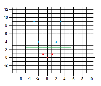
Example 2: 3 points in a plane

Points and class (coordinate x (x1), coordinate y (x2), class/output (y)):
![x = [-1,-1]](https://s0.wp.com/latex.php?latex=x+%3D+%5B-1%2C-1%5D&bg=ffffff&fg=000&s=0&c=20201002)
Class (output):
Point 2:
![x = [2,0]](https://s0.wp.com/latex.php?latex=x+%3D+%5B2%2C0%5D&bg=ffffff&fg=000&s=0&c=20201002)
Class (output):
Point 3:
![x = [3,1]](https://s0.wp.com/latex.php?latex=x+%3D+%5B3%2C1%5D&bg=ffffff&fg=000&s=0&c=20201002)
Class (output):
First let us calculate the second part of the function we want to minimize. You can see both alphas being multiplied by two numbers. The first number is the product of 


![w = 1*-1*[-1,-1] + 3*1*[2,0] - 2*1*[3,1] = [1,-1] \\<br /> b_1 = b_2 = b_3 = -1](https://s0.wp.com/latex.php?latex=w+%3D+1%2A-1%2A%5B-1%2C-1%5D+%2B+3%2A1%2A%5B2%2C0%5D+-+2%2A1%2A%5B3%2C1%5D+%3D+%5B1%2C-1%5D+%5C%5C%3Cbr+%2F%3E+b_1+%3D+b_2+%3D+b_3+%3D+-1&bg=ffffff&fg=000&s=0&c=20201002)
Result:

Appendix A: Scalar Projection of Vectors
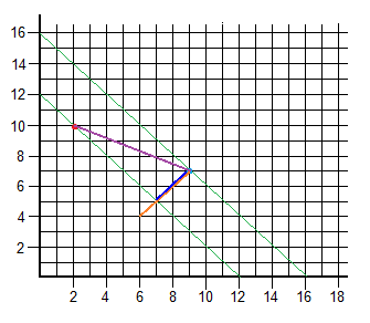
We have two points and its vector:
![R = [2,10] \quad \text{(red)} \\<br /> B = [9,7] \quad \text{(blue)} \\<br /> \overrightarrow{RB} = (7,-3)](https://s0.wp.com/latex.php?latex=R+%3D+%5B2%2C10%5D+%5Cquad+%5Ctext%7B%28red%29%7D+%5C%5C%3Cbr+%2F%3E+B+%3D+%5B9%2C7%5D+%5Cquad+%5Ctext%7B%28blue%29%7D+%5C%5C%3Cbr+%2F%3E+%5Coverrightarrow%7BRB%7D+%3D+%287%2C-3%29&bg=ffffff&fg=000&s=0&c=20201002)
And we want to calculate the length of the vector’s projection (purple) on the orange vector 
For this, we have to solve the formula:

Now with the length and the angle, we can calculate the coordinates using sine and cosine functions.

B was in [9,7], so the point on the other side of the projection is
![[9-2,7-2] \to [7,5]](https://s0.wp.com/latex.php?latex=%5B9-2%2C7-2%5D+%5Cto+%5B7%2C5%5D+&bg=ffffff&fg=000&s=0&c=20201002)
Appendix B: Lagrange Multipliers
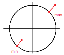
Lagrange is a strategy to find local maxima and minima of a function subject to equality constraints, i.e. max of 


If 


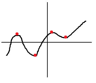
| In mathematics, a stationary point of a differentiable function of one variable is a point of the function domain where the derivative is zero. For a function of several variables, the stationary point is an input whose all partial derivatives are zero (gradient zero). They correspond to local maxima or minima. |
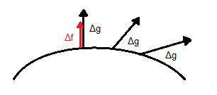
To make it clear, let us say that we have a surface  whose gradient is whose gradient is  and it is perpendicular to the whole surface. We try to find its maxima whose gradient should theoretically be perpendicular as well. Let us not forget the relationship between the first derivative and the gradient. Hence we can say that the gradient of and it is perpendicular to the whole surface. We try to find its maxima whose gradient should theoretically be perpendicular as well. Let us not forget the relationship between the first derivative and the gradient. Hence we can say that the gradient of  and the gradient of and the gradient of  are pointing in the same direction so: are pointing in the same direction so:  (proportional). is called Lagrange multiplier. (proportional). is called Lagrange multiplier.
|
Example 1: 1 constraint, 2 dimensions
Maximize 


Now we plug these results into the original equation.

Therefore we have two points:

Example 2: 1 constraint, 2 dimensions
Find the rectangle of maximal perimeter that can be inscribed in the ellipse 


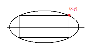

Now plug it into the original equation.

Then,
So the maximum permieter is:


Example 3: 2 constraints, 3 dimensions


Now plug it into 


Since this is a parabola in 3 dimensions, this has no maximum, so it is a minimum.


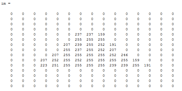
![Channel_{red} = [0 \quad 237 \quad 237] \\<br /> Channel_{green} = [0 \quad 28\quad 28] \\<br /> Channel_{blue} = [0 \quad 36 \quad 36]](https://s0.wp.com/latex.php?latex=Channel_%7Bred%7D+%3D+%5B0+%5Cquad+237+%5Cquad+237%5D+%5C%5C%3Cbr+%2F%3E+Channel_%7Bgreen%7D+%3D+%5B0+%5Cquad+28%5Cquad+28%5D+%5C%5C%3Cbr+%2F%3E+Channel_%7Bblue%7D+%3D+%5B0+%5Cquad+36+%5Cquad+36%5D&bg=ffffff&fg=000&s=0&c=20201002)
![Pixel_{5,8} = [237 \quad 28 \quad 36]](https://s0.wp.com/latex.php?latex=Pixel_%7B5%2C8%7D+%3D+%5B237+%5Cquad+28+%5Cquad+36%5D&bg=ffffff&fg=000&s=0&c=20201002)


 (desired output minus system’s output) but in MLP the squared error function will be used instead
  :
: to make it simpler when obtaining the derivative.
 Input matrix.
 Weights’ matrix that connects the input and hidden layers.
 Weights’ matrix that connects the hidden and output layers.
 Desired output.
 Learning rate.
 Content of each node in the hidden layer (before activation).
 Content of each node in the hidden layer (after activation).
 Content of each node in the output layer (before activation).
 MLP output.
 Squared error function.
 . For this, it is necessary to calculate the derivative of the error with respect to
![\frac{1}{2} \cdot 2 \cdot (y - \widehat{y}) \cdot [ \frac{\partial y}{\partial W_2} - \frac{\partial \widehat{y}}{\partial W_2} ]](https://s0.wp.com/latex.php?latex=%5Cfrac%7B1%7D%7B2%7D+%5Ccdot+2+%5Ccdot+%28y+-+%5Cwidehat%7By%7D%29+%5Ccdot+%5B+%5Cfrac%7B%5Cpartial+y%7D%7B%5Cpartial+W_2%7D+-+%5Cfrac%7B%5Cpartial+%5Cwidehat%7By%7D%7D%7B%5Cpartial+W_2%7D+%5D&bg=ffffff&fg=000&s=0&c=20201002)


 the procedure is very similar:
![\frac{\partial J}{W_1} = [\text{same things...} ] = \delta_3 \cdot \frac{\partial z_3}{\partial W_1} = \delta_3 \cdot \frac{\partial z_3}{\partial a_2} \cdot \frac{\partial a_2}{\partial W_1} \\<br /> = \delta_3 \cdot W_2 \cdot \frac{\partial a_2}{\partial z_2} \cdot \frac{\partial z_2}{\partial W_1} = \delta_3 \cdot W_2 \cdot f'(z_2) \cdot x](https://s0.wp.com/latex.php?latex=%5Cfrac%7B%5Cpartial+J%7D%7BW_1%7D+%3D+%5B%5Ctext%7Bsame+things...%7D+%5D+%3D+%5Cdelta_3+%5Ccdot+%5Cfrac%7B%5Cpartial+z_3%7D%7B%5Cpartial+W_1%7D+%3D+%5Cdelta_3+%5Ccdot+%5Cfrac%7B%5Cpartial+z_3%7D%7B%5Cpartial+a_2%7D+%5Ccdot+%5Cfrac%7B%5Cpartial+a_2%7D%7B%5Cpartial+W_1%7D+%5C%5C%3Cbr+%2F%3E+%3D+%5Cdelta_3+%5Ccdot+W_2+%5Ccdot+%5Cfrac%7B%5Cpartial+a_2%7D%7B%5Cpartial+z_2%7D+%5Ccdot+%5Cfrac%7B%5Cpartial+z_2%7D%7B%5Cpartial+W_1%7D+%3D+%5Cdelta_3+%5Ccdot+W_2+%5Ccdot+f%27%28z_2%29+%5Ccdot+x&bg=ffffff&fg=000&s=0&c=20201002)

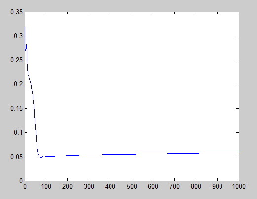
 is too big, it can escape from the minimum with an unknown result. In this case, it resulted absolutely good, but it is not always the case.
 . Right:
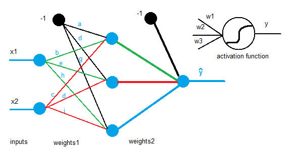
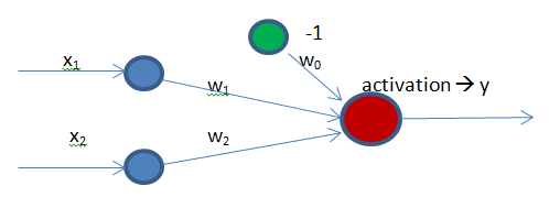
![input = [0.245 \quad 0.942 \quad 0.441] \\<br /> weights = [0.1 \quad 0.32 \quad 0.63 \quad 0.04] \\<br /> sum = -1*0.1 + 0.245*0.1 + 0.942*0.32 + 0.942*0.63 + 0.441*0.04 \\<br /> class = activation(sum) \\](https://s0.wp.com/latex.php?latex=input+%3D+%5B0.245+%5Cquad+0.942+%5Cquad+0.441%5D+%5C%5C%3Cbr+%2F%3E+weights+%3D+%5B0.1+%5Cquad+0.32+%5Cquad+0.63+%5Cquad+0.04%5D+%5C%5C%3Cbr+%2F%3E+sum+%3D+-1%2A0.1+%2B+0.245%2A0.1+%2B+0.942%2A0.32+%2B+0.942%2A0.63+%2B+0.441%2A0.04+%5C%5C%3Cbr+%2F%3E+class+%3D+activation%28sum%29+%5C%5C&bg=ffffff&fg=000&s=0&c=20201002)
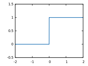
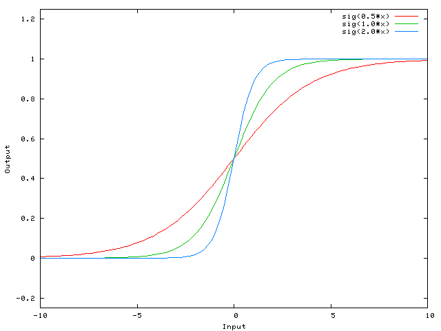
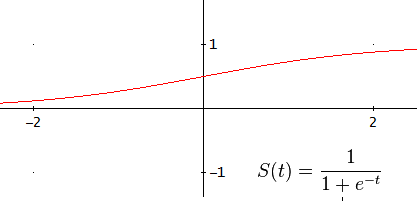
 dependent argument, the steepness of the sigmoid function can be modified. However, it cannot go anywhere further than 0 when the input is 0. For this, we need a bias.
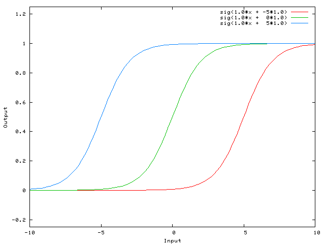


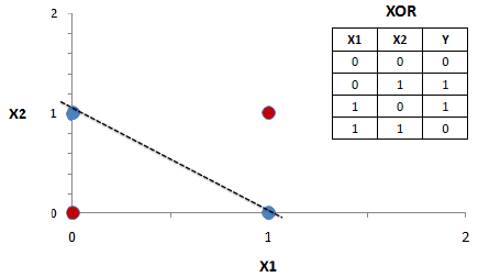

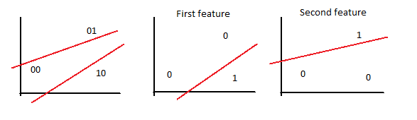
 . The 00 class would be class A, 01 class B, and so on. Nonetheless, the weights which go from input neurons to a certain output are able to classify just one element, so if 4 different classes are aimed to be distinguished, the same number of output neurons are needed.


 .
.
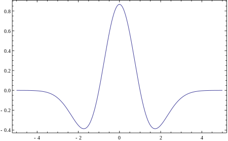
 generate a kernel


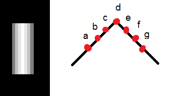
 , kernel’s size = 7


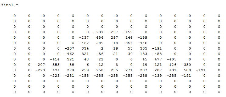
 which is the separation between points. This operation reveals that this error can be reduced by spacing the differenced points by one pixel (averaging tends to reduce noise). This is equivalent to computing the first order difference viewed in the previous formula at two adjacent points, as a new difference where:


You must be logged in to post a comment.