Recently I was reading up on an interesting paper that explores how colorizing black and white images using Deep Learning. The paper was easy to read and understand, and to fully enjoy it I decided to implement it in a lower scale. I have a laptop with a humble graphic card and an i7 so it cannot compete with those servers that cost several thousand euros, that is why I have not focused on the design of the network but more on the algorithmic part.
Goals and dataset
The goals of this post are:
- To be able to implement the algorithm to learn about a new colorizing approach.
- To have a look to the neural network they used.
- To figure out if a simpler network can learn even if the results are quite improvable.
- To practice using tensorflow.
- To have fun.
The dataset I will use can be downloaded here. It consist of 2687 256×256 images of beaches, forests, streets, etc.
Algorithm
One of the things I enjoyed about the paper [1] is how well structured it is, which made the understanding much easier. I will try to follow their structure in a similar way while being precise and concise.
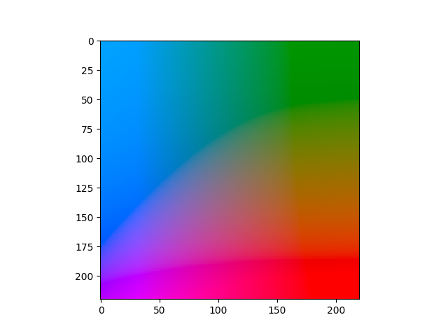
The very first important thing we need to know is that Lab color space is used. The reason is simple: in color spaces such as RGB we need to learn three different channels whereas in Lab we only need to learn two. The channel L refers to the lightness, having values between 0 (dark) and 100. The channels a and b are the position in the axis between red-green and blue-yellow respectively.

A typical approach would use the L channel as input and the a,b channels as output (for every pixel the prediction consists on two values). However, they argue that using a loss function based on two components does not represent the multimodal and ambiguity problems properly. We are surrounded by objects that can have multiple colors such as apples since they can be red, green or yellow. In addition, Euclidian distance (averaging) will increase desaturated (grayish) values.
In order to solve this they divided the a,b colorspace into Q bins corresponding to probabilities, and consequently, the number of predictions expected per pixel will be Q (one per bin). For instance, in case of the apple, the bins corresponding to red, yellow and green will contain higher probabilities than those bins close to colors like blue.
I skipped representing some bins by analyzing first the colors I have in my dataset so that I only take into account those bins with colors used in my dataset. My a,b color space is between -110 and 110 and depending on the size of the squared window used to divide it, the resulting grid and the final used bins will be different. When I’m using the whole dataset and a window size of 10 I use XX bins and it raises to XXX bins when the window size is 5. In contrast, the authors use Q=313 bins.
The problem is now a simple classification problem in which we have an input (brightness values) and the output is a set of probabilities indicating how likely are the values to belong to a certain bin. A classic way to solve this is to use cross entropy but in addition to it, the authors noticed that the model is biased towards low a,b values which typically correspond to backgrounds such as walls, sky, etc. In order to solve this, they rebalanced the colors by adding weights that will multiply the cross entropy calculated.
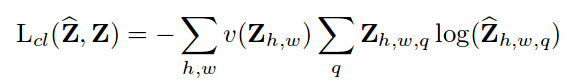
This formula can be read as: perform cross-entropy on a pixel comparing the original and predicted distribution of the probabilities, and then multiply it by a weight corresponding to that color such that certain colors are highlighted to the network.
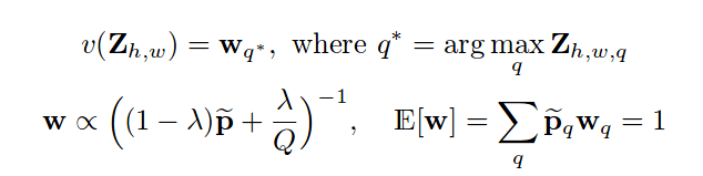
To calculate these weights they introduced a new hyper-parameter 


In the image above, the left side shows that the most used colors are located in the center (desaturated) and both cases differ depending on the dataset: when only forest images were used, less pink-red colors were used.
This is basically all, in regards to the training part. The other important issue arises when predicting values. Imagine for a second that for a single pixel the network spits a probability distribution such that all values are zero except for one value that is one (the so called one-hot vector). It is more than clear that the corresponding bin will represent the color of that pixel. Nonetheless, we will probably have several probabilities and mapping them back to a,b values is the next task. They introduced a new variable called T standing for temperature (coming from simulated annealing). To put it simple, when T tends to zero, values are more intense since the prediction emphasizes the color with the highest probability. On the other hand, when T tends to one, the colors are more distributed but also more desaturated because the color is result of a more spread average of the obtained probabilities.
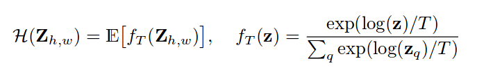
The formula above describes how they calculated the prediction given the temperature T and the distribution z.
Neural Network
As I have mentioned before, due to my limited resources, utilizing the network they used was immediately discarded. Thus I designed a very simple neural network that consists of 8 convolutional layers. The input consist of a window of 32×32 pixels and after the convolutions the final prediction has a size of 16×16. In every convolution the size is reduced by 2 because of the 3×3 kernel thus reducing one pixel on each side of the image. The number of filters used depends on the number of bins Q such that they are growing using a step of Q/8. For instance, the number of filters in the first convolutional layer is Q/8, in the second layer is 2*Q/8, and so on until the last layer with a number of Q filters. Therefore, the size of my final output will be 16x16xQ.
Results
At first I was using only the forest dataset to speed up the training process and regardless of some hyper-parameters tunning the results were a bit random: sometimes they were quite okay and sometimes they were bad, but in all cases the network was learning and showing a behavior that makes sense, so I can say that I am satisfied with the results.

The code is provided in the Source code section.
References
1. Zhang R., Isola P. & Efros A.A. 2016. Colorful Image Colorization.