[Explanation] Face Recognition using Eigenfaces

This post comes from an assignment for my “Cognitive Science I” course. Enjoy it.

Brief Introduction

This paper is one of the most relevant papers regarding to face recognition. Nowadays it is difficult to find a real life implementation of this old algorithm, but other research has been built upon this. In addition, the simplistic and effectiveness of this algorithm makes it very beautiful.

Algorithm

To train the model:
1.-Flat the black and white images of the training set (from matrices to vectors)
2.-Calculate the mean.
3.-Normalize the training set: for each image, subtract the mean.
4.-Calculate the covariance: multiply all images by themselves.
5.-Extract eigenvectors from the covariance.
6.-Calculate eigenfaces: eigenvectors x normalized pictures.
7.-Choose the most significant eigenfaces.
8.-Calculate weights: chosen eigenfaces x normalized pictures.

To detect a face:
9.-Vectorize and normalize this picture: subtract the calculated mean from the picture.
10.-Calculate the weights: multiply the eigenfaces x normalized picture.
11.-Interpret the distance of this weight vector in the face space: if it is far, it is not a face (establishment of a threshold).

Explanation of the algorithm

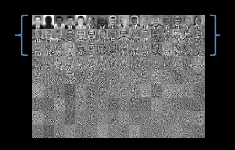
Training set used:

1.-Flatting the image
This algorithm works with vectors because we have to calculate later the covariance. Because of this, the image needs to be in a vector form.

1 2 3 4 5 6 7 8 9

1 4 7 2 5 8 3 6 9

2.-Calculate the mean
The mean is just the sum of all of the pictures divided by the number of pictures. As a result, we will have an “average” face.

3.-Normalize the training set
To normalize the training set, we just simply need to subtract for each picture in the training set the mean that was calculated in the previous step.

The reason why this is necessary is because we want to create a system that is able to represent any face. Therefore, we calculated the elements that all faces have in common (the mean). If we extract this average from the pictures, the features that distinguish each picture from the rest of the set are visible.

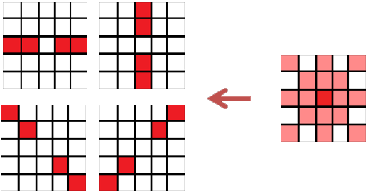
4.-Calculate the covariance
The covariance represents how two variables change together. After the previous step, we have a set of images that have different features, so now we want to see how these features for each individual picture change in relation to the rest of the pictures.

For this purpose, we put all the flat normalized pictures together in a vector. My training set consists of 16 pictures whose dimensions are 235×235 pixels. Therefore, the resulting matrix will be 55225×16. The covariance is the multiplication of this matrix by itself, and if we transpose it correctly, the resulting matrix will be 16×16:

16x55225 * 55225x16 = 16×16

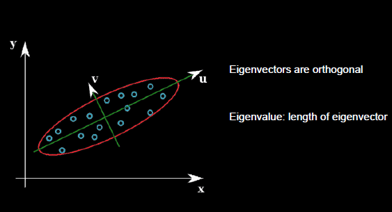
5.-Extract eigenvectors
From the covariance we can extract the eigenvectors. Fortunately, there is Matlab function that helps us in this step (you can see it on the code). There is plenty of information in the internet about eigenvectors (2) (3) but the general idea is that eigenvectors are the vectors of the covariance that describe the direction of the data. The first eigenvector will describe more information than the second and so on. For this reason, later we have to pick the first eigenvectors generated (avoiding noise).

6.-Calculate eigenfaces
Each eigenvector is multiplied by the whole normalized training set matrix (the 55225×16 matrix) and as a result, we will have the same amount of eigenfaces as images in our training set.

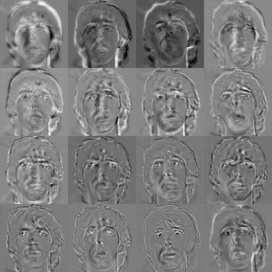
7.-Choose the most significant eigenfaces.
The first eigenfaces represent more information than the last eigenfaces. Actually, the last eigenfaces only add noise to the model, so it is necessary to avoid them. Therefore, only the most significant eigenfaces are chosen. For this, there are many heuristic algorithms but it can also be done by looking at the pictures. In my code I only used 16 different pictures, and since the training set is tiny, all of the eigenfaces represent important features.

Some simple heuristic algorithms are shown in the code but they are not used. I preferred to manually select the amount of eigenfaces to see the difference in the algorithm’s performance.

Among these heuristics are:
1) To select those eigenvectors whose eigenvalues are above 1.
2) To choose all eigenvectors until the cumulative sum of the eigenvalues is around 95%

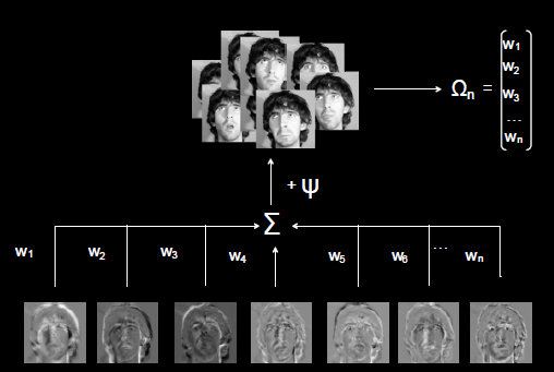
8.-Calculate weights
Each normalized face in the training set multiplies each eigenface. Consequently, there will be N set of weights with M elements (N = amount of pictures in the training set, M = number of eigenfaces).

After this procedure, we can theoretically represent each face as a linear combination of the chosen eigenfaces. This means that each picture in the training set can be recalculated by a sum of each eigenface multiplied by the corresponding weight plus the mean.

Recognition part: 9.-Vectorize and normalize the picture
Reshape the test picture into a vector and subtract the mean calculated in 2) from it.

Recognition part: 10.-Calculate the weights
The same as 8) but with the test picture.

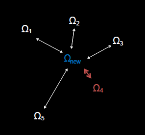
Recognition part: 11.-Interpret the distance
Now we have all the weights from our training set and the weight of the picture that we want to classify. The final step is to determine whether the picture is a face or not, given the distance. This can be a bit confusing: the most obvious approach might be calculate the mean of the distances and if the distance is over a predetermined threshold, the picture will be categorized as a face. Nonetheless, this might lead to errors when using, for example, one of the faces used in the training set.

Since the model was trained using the same image, for the system should be obvious to categorize this picture as a face. Unfortunately, that is not the case. The reason is because the distance of the picture used in the training regarding to the specific eigenface that describes its features might be 0 (because it is exactly the same picture) but the distances between this picture and the rest of the images in the training set might be greater, and if we take the mean of the distances, the overall result could be over the threshold that we determined.

The code is provided in the Source code section.
You can also access to the slides of the presentation.

References

1. Matthew A. Turk & Alex P. Pentland. 1991. “Face recognition using Eigenfaces”.
2. “Principal Component Analysis 4 Dummies: Eigenvectors, Eigenvalues and Dimension Reduction”. https://georgemdallas.wordpress.com/2013/10/30/principal-component-analysis-4-dummies-eigenvectors-eigenvalues-and-dimension-reduction/ (Accessed 5-10-2015)
3. Eigenvectors and Eigenvalues Explained Visually. http://setosa.io/ev/eigenvectors-and-eigenvalues/ (Accessed 5-10-2015)