Brief Introduction
Hough Transform was already used for Line detection and it showed how powerful it can be. This time, the main goal will be detecting circles. Detecting this basic shape may be interesting in the field of recognition since many objects subject to be classified have a circular shape such as the iris of the eyes, coins or even cells under a microscope.

Simple way (3 dimensional matrix)
This first method is easier to understand but very inefficient compared to the next (after space reduction is applied). A circle needs three parameters: x,y values for the center location and the radius of the circumference. Thus the accumulator matrix will have 3 dimensions, one for each parameter, covering all possibilities.
Given a certain radius, when a pixel is detected, the algorithm will increment the accumulator elements corresponding to the circumference that can be drawn using that pixel and radius as characteristics of the circle.
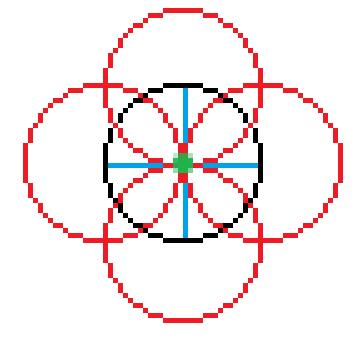
The first two parameters of the 3-D accumulator are x,y values corresponding to the coordinates of the whole picture. The third parameter is the radius. In the following picture, we are using a fixed radius to make everything easier to understand, and the accumulator is incremented in those coordinates in which a red pixel is located.

As you can see, the red pixels almost do not coincide in any point when iterating over the same coordinate. During the algorithm execution, many circles will be drawn and there will be a peak in the center of the real circle we want to detect, as depicted below. They all meet in the center of the circumference (green points).
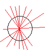
When the algorithm finishes the iteration over all pixels and radius, we only need to find where is that maxima located to get the characteristics of the circumference. Finally, we can draw it.

The most problematic characteristic of this algorithm is that it needs to iterate over all radius, so it will lose a considerable amount of time on this task. For this reason, in the algorithm I developed I establish a min and max radius, to avoid checking radius extremely short and radius too large. This is how it looks depending on the described situation.
 |
 |
 |
||
| a) | b) | c) |
a) When the circumference has a larger radius than expected.
b) When it finds more figures.
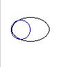
c) When it only finds an ellipse.
The algorithm is this:
Iterate over columns (x)
Iterate over rows (y)
If an edge is detected
Iterate over all radius (r)
For angles between 0 and 360 (m)
Calculate pixel for the generated circumference (y,x,r)
If that pixel is not out of bounds, increase accumulator
Space Reduction
Space reduction in this case consist in removing the problematic radius parameter.
When iterating over the picture and a pixel is detected, it will try to look for more pixels in a enclosed neighborhood. When a pixel in the neighborhood is detected, we will have an arc of the circumference. Given these two pixels, we will have a slope and a middle point (blue). We need to find the perpendicular line passing through that middle point (red) which represents the increment in the accumulator.

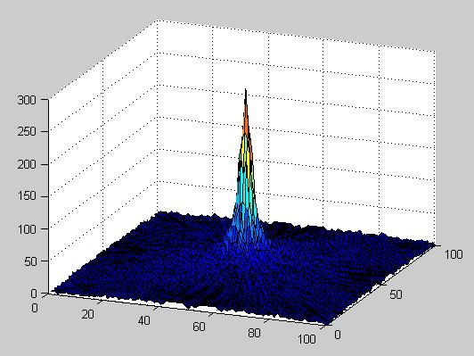
As the algorithm iterates, it will increase more and more the accumulator, and a peak in the center of the real circumference will be generated.
 |
 |
|
| After some iterations | Accumulator plotted |
There is another method to obtain the center explained in [1], but the algorithm written in the book is an implementation of the already explained method. However, the author of the books does not give a hint about getting the radius once we got the center.
I used a 1 dimensional array (or vector) as an accumulator of the distances of each pixel in the image to the center. The peak will be generated when the distances of all the pixels belonging to the circumference are summed in the accumulator. This results in the radius of that circumference. It may be improved by starting in the neighborhood of the center and stop counting at some point.
The execution time differs from the improved algorithm and from the non-improved algorithm. For the same picture, the non-improved algorithm takes around 0.39 seconds whereas the improved version takes around 0.019 seconds.
The code is provided in the Source code section.
References
1. M. Nixon and A. Aguado. 2008. “First order edge detection operators”, Feature Extraction & Image Processing.
One thought to “[Hough Transform] Circle detection and space reduction”