[Supervised Learning] SVM – Support Vector Machine explained with examples

This post is the first part of a double post about SVMs. This part tries to help to clarify how SVMs work in theory (with 2 full developed examples). The second part (not published yet) will explain the algorithm to solve this problem using a computer: Quadratic Programming and SMO.

Index

• Basic definition of SVMs for binary classification
• Mathematical explanation
• Kernel trick
• Example 1: 2 points in a plane
• Example 2: 3 points in a plane
• Appendix A: Scalar Projection of Vectors (1 example)
• Appendix B: Lagrange Multipliers (3 examples)

Basic definition

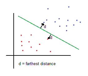
Support vector machines (SVMs from now on) are supervised learning models used for classification and regression. The basic idea of SVMs in binary classification is to find the farthest boundary from each class.

Therefore, solving a basic mathematical function given the coordinates (features) of each sample will tell whether the sample belongs to one region (class) or other. Input features determine the dimension of the problem. To keep it simple, the explanation will include examples in 2 dimensions.

Mathematical explanation

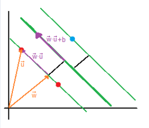
The vector [latex]\overrightarrow{w}[/latex] is a perpendicular vector to the boundary, but since boundary’s coefficients are unknown, [latex]\overrightarrow{w}[/latex] vector’s coefficients are unknown as well. What we want to do is to calculate the boundary’s coefficients with respect to [latex]\overrightarrow{u}[/latex] because we have its coordinates (sample’s coordinates).

If both vectors are multiplied, the result will be the purple vector. [latex]\overrightarrow{w} \cdot \overrightarrow{u} \geq c \quad \text{or generally} \quad \overrightarrow{w} \cdot \overrightarrow{u} + b \geq 0[/latex]

Let us say that:
[latex]\overrightarrow{w} \cdot \overrightarrow{x_+} + b \geq 1 \quad \text{and} \quad \overrightarrow{w} \cdot \overrightarrow{x_-} + b \leq -1[/latex]
Where [latex]\overrightarrow{x_+}[/latex] is a positive sample (class A) and [latex]\overrightarrow{x_-}[/latex] is a negative sample (class B).
A new variable is now introduced:
[latex]y_i \quad \text{such that } y_i = +1 \quad \text{for + samples} \\
\text{ } \hspace{70pt} y_i = -1 \quad \text{for – samples}[/latex]

Multiply each of them by the previous equations:
[latex]y_i(\overrightarrow{x_i} \cdot \overrightarrow{w}+b) \geq 1 \\
+1 * (\overrightarrow{x_i} \cdot \overrightarrow{w}+b) \geq 1 \\
-1 * (\overrightarrow{x_i} \cdot \overrightarrow{w}+b) \geq 1[/latex]

The result is the same equation. Therefore, we only need the previous formula:
[latex]y_i(\overrightarrow{x_i} \cdot \overrightarrow{w}+b) \geq 1 \quad \to \quad y_i(\overrightarrow{x_i} \cdot \overrightarrow{w}+b) -1 \geq 0[/latex]

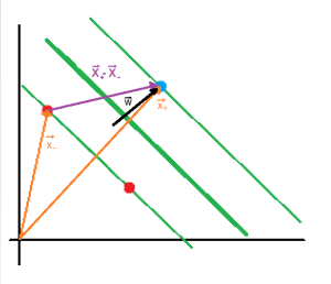
Finally, we add an additional constrain [latex]y_i(\overrightarrow{x_i} \cdot \overrightarrow{w}+b) -1 = 0[/latex] so that the values that fulfill this, fall in between the two regions as depicted (green zone).

The next step is to maximize the projection of [latex]\overrightarrow{x_+}-\overrightarrow{x_-}[/latex] on [latex]\overrightarrow{w}[/latex] (the black perpendicular vector to the boundary) to keep samples from each class as far as possible. I assume that you know about scalar projection, but if you don’t, you can check out the Appendix A. The length of the projection is given by the following formula: [latex](x_+ – x_-) \cdot \frac{\overrightarrow{w}}{\| w \|}[/latex]

From the previous formula [latex]y_i(\overrightarrow{x_i} \cdot \overrightarrow{w}+b) -1 = 0[/latex] now let us substitute both positive and negative samples [latex]x_+[/latex] and [latex]x_-[/latex] so that:
[latex]y_i = +1 \quad \to \quad 1(\overrightarrow{x_+} \cdot \overrightarrow{w} + b) -1 = 0 \quad \to \quad \overrightarrow{x_+} \cdot \overrightarrow{w} = 1-b \\
y_i = -1 \quad \to \quad -1(\overrightarrow{x_-} \cdot \overrightarrow{w} + b) -1 = 0 \quad \to \quad \overrightarrow{x_-} \cdot \overrightarrow{w} = -1-b [/latex]

Therefore:
[latex](x_+ – x_-) \cdot \frac{\overrightarrow{w}}{\| w \|} = \frac{\overrightarrow{x_+} \cdot \overrightarrow{w}-\overrightarrow{x_-} \cdot \overrightarrow{w}}{\| w \|} = \frac{1-b+1+b}{\| w \|} = \frac{2}{\| w \|}[/latex]

The goal is to maximize [latex]\frac{2}{\| w \|}[/latex] which is the same as minimizing [latex]\| w \|[/latex] or, to make it more mathematically convenient, [latex]\frac{1}{2}\| w \|^2[/latex]

Thus, we have a function to minimize with a constraint ([latex]y_i(\overrightarrow{x_i} \cdot \overrightarrow{w} + b) -1 = 0 [/latex]), so Lagrange is applied. In case you want to know more about Lagrange multipliers, you can check Appendix B.

[latex]L = \frac{1}{2}\| w \|^2 – \sum \alpha_i [ y_i (\overrightarrow{w} \cdot \overrightarrow{x_i} +b)-1][/latex]
First we have the function we want to minimize, and later the constraints.

[latex]\frac{\partial L}{\partial w} = \overrightarrow{w} – \sum \alpha_i y_i x_i = 0 \to \overrightarrow{w} = \sum \alpha_i y_i x_i \\
\frac{\partial L}{\partial b} = – \sum \alpha_i y_i = 0 \to \sum \alpha_i y_i = 0[/latex]

Plug these two functions to [latex]L[/latex].

[latex]L = \frac{1}{2}(\sum \alpha_i y_i \overrightarrow{x_i}) \cdot (\sum \alpha_j y_j \overrightarrow{x_j}) – (\sum \alpha_i y_i \overrightarrow{x_i}) \cdot (\sum \alpha_j y_j \overrightarrow{x_j}) – \sum \alpha_i y_i b + \sum \alpha_i = \sum \alpha_i – \frac{1}{2} \sum_i \sum_j \alpha_i \alpha_j y_i y_j \overrightarrow{x_j} \cdot \overrightarrow{x_j}[/latex]

Hence, we aim to minimize [latex]\sum \alpha_i – \frac{1}{2} \sum_i \sum_j \alpha_i \alpha_j y_i y_j \overrightarrow{x_j} \cdot \overrightarrow{x_j}[/latex]
The optimization depends on [latex]\overrightarrow{x_j} \cdot \overrightarrow{x_j}[/latex]

Kernel trick

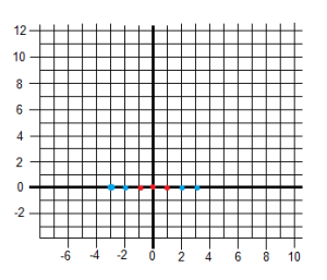
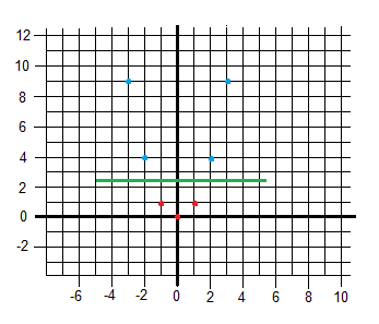
One of the most interesting properties of SVMs is that we can transform problems from a certain number of dimensions to another dimensional space. This flexibility, as known as kernel trick, allows SVMs to classify nonlinear problems.

[latex]\text{from } \quad f(x) \quad \text{ to } \quad f(x,x^2)[/latex]

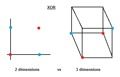
The following example shows how to graphically solve the XOR problem using 3 dimensions.

Now it is not difficult to imagine a plane that can separate between blue and red samples.

Example 1: 2 points in a plane

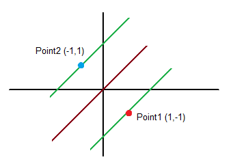
Points and class (coordinate x (x1), coordinate y (x2), class/output (y)):

We want to minimize: [latex]\sum_{i=1}^N \alpha_i – \frac{1}{2} \sum_{i=1}^N \sum_{i=1}^N \alpha_i \alpha_j y_i y_j x_i^T \cdot x_j[/latex]
We know that: [latex]w = \sum_{i=1}^N \alpha_i y_i x_i[/latex]
and [latex]\sum_{i=1}^N \alpha_i y_i = 0[/latex]

Let us calculate the second part of the function we want to minimize first to keep it simple:
[latex]
L_1 = \begin{cases} \alpha_1 * \alpha_1 * 1 * 1 * (-1 * -1 + 1*1) = 2 \alpha_1^2\\
\alpha_1 * \alpha_2 * 1 * -1 * (-1 * 1 + 1*-1) = 2 \alpha_1 \alpha_2 \\
\alpha_2 * \alpha_1 * -1 * 1 * (1 * -1 + -1*1) = 2 \alpha_1 \alpha_2 \\
\alpha_2 * \alpha_2 * -1 * -1 * (1 * 1 + -1*-1) = 2 \alpha_2^2 \end{cases} = 2 \alpha_1^2 + 2 \alpha_1 \alpha_2 + 2 \alpha_1 \alpha_2 + 2 \alpha_2 \\
[/latex]

[latex]L = \alpha_1 + \alpha_2 – \frac{1}{2} (2 \alpha_1^2 + 2 \alpha_1 \alpha_2 + 2 \alpha_1 \alpha_2 + 2 \alpha_2) = \alpha_1 + \alpha_2 – 2 \alpha_1 \alpha_2 – \alpha_1^2 – \alpha_2^2[/latex]

[latex]
\vspace{2 em}
\frac{\partial L}{\partial \alpha_1} = 0 \quad \to \quad -2 \alpha_1 – 2 \alpha_2 +1 = 0 \quad \to \quad \alpha_1 + \alpha_2 = \frac{1}{2} \\
\frac{\partial L}{\partial \alpha_2} = 0 \quad \to \quad -2 \alpha_2 – 2 \alpha_1 +1 = 0 \quad \to \quad \alpha_1 + \alpha_2 = \frac{1}{2} [/latex]

[latex]
\vspace{2 em}
\sum_{i=1}^N \alpha_i y_i = 0 \quad \to \quad 1 \alpha_1 – 1 \alpha_2 = 0 \quad \to \quad \alpha_1 = \alpha_2
[/latex]

Ergo:

[latex]\alpha_1 = \alpha_2 = \frac{1}{4}[/latex]

Now let us calculate [latex]\overrightarrow{w}[/latex]:

[latex]\overrightarrow{w} = \sum_{i=1}^N \alpha_i y_i x_i = \frac{1}{4} * 1 * [-1,1] + \frac{1}{4} * -1 * [1,-1] = [\frac{-1}{4} , \frac{1}{4}] + [\frac{-1}{4} , \frac{1}{4}] = [\frac{-2}{4} , \frac{2}{4}] = [\frac{-1}{2} , \frac{1}{2}][/latex]

Now we have to figure out the bias
[latex]\alpha [y_i (\overrightarrow{w}^T\overrightarrow{x_i} +b) -1] = 0 \quad \to \quad \alpha_i y_i \overrightarrow{w}^T\overrightarrow{x_i} + \alpha_i b y_i – \alpha_i = 0 \\
b = \frac{1-y_i \overrightarrow{w}^T\overrightarrow{x_i}}{y_i} \quad \to \quad b = \frac{1}{y_i} – \overrightarrow{w}^T\overrightarrow{x_i}[/latex]

[latex]
\text{for i=1} \\
\text{ } \hspace{3em} b = 1 -[(-1,1) \cdot (\frac{-1}{2},\frac{1}{2})] = 0 \\
\text{for i=2} \\
\text{ } \hspace{3em} b = – 1 -[(1,-1) \cdot (\frac{-1}{2},\frac{1}{2})] = 0
\vspace{3em}
\text{ }[/latex]

Solution = [latex]\frac{-1}{2}x+\frac{1}{2}y=0 \quad \to \quad x-y=0[/latex]

Example 2: 3 points in a plane

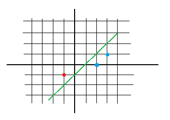
Points and class (coordinate x (x1), coordinate y (x2), class/output (y)):

First let us calculate the second part of the function we want to minimize. You can see both alphas being multiplied by two numbers. The first number is the product of [latex]y_i[/latex] and [latex]y_j[/latex]. The second number is the dot product between the two coordinates [latex]\overrightarrow{x_i} \cdot \overrightarrow{x_j}[/latex].
[latex]
L_1 = \begin{cases} \alpha_1 * \alpha_1 * 1 * 2\\
\alpha_1 * \alpha_2 * -1 * -2 \\
\alpha_2 * \alpha_1 * -1 * -4 \\
\alpha_2 * \alpha_2 * -1 * -2 \\
\alpha_1 * \alpha_2 * 1 * 4 \\
\alpha_2 * \alpha_1 * 1 * 6 \\
\alpha_2 * \alpha_2 * -1 * -4 \\
\alpha_1 * \alpha_2 * 1 * 6 \\
\alpha_2 * \alpha_1 * 1 * 10 \end{cases} = 2 \alpha_1^2 + 4 \alpha_1 \alpha_2 + 8 \alpha_1 \alpha_3 + 4 \alpha_2^2 + 12 \alpha_2 \alpha_3 + 10 \alpha_3^2 = 0 \\
\text{Apply } \alpha_1 = \alpha_2 + \alpha_3 \text{ and } \frac{-1}{2} \\
2 \alpha_2 + 2 \alpha_3 – 5 \alpha_2^2 – 10 \alpha_3^2 – 14 \alpha_2 \alpha_3 = 0
\vspace{1em}
\text{  }
[/latex]

[latex]
\frac{\partial L}{\partial \alpha_2} = 2 – 10 \alpha_2 – 14 \alpha_3 = 0 \\
\frac{\partial L}{\partial \alpha_3} = 2 – 14 \alpha_2 – 20 \alpha_3 = 0 \\
\alpha_2 = 3, \alpha_3 = -2, \alpha_1 = 1
[/latex]

[latex]w = 1*-1*[-1,-1] + 3*1*[2,0] – 2*1*[3,1] = [1,-1] \\
b_1 = b_2 = b_3 = -1[/latex]

Result: [latex]x – y -1 = 0[/latex]

Appendix A: Scalar Projection of Vectors

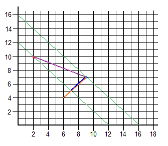
We have two points and its vector:
[latex]R = [2,10] \quad \text{(red)} \\
B = [9,7] \quad \text{(blue)} \\
\overrightarrow{RB} = (7,-3)[/latex]

And we want to calculate the length of the vector’s projection (purple) on the orange vector [latex]\overrightarrow{O}[/latex] (which by the way, is the perpendicular of both green lines). The result is the blue vector which is over the orange one within the green region.

For this, we have to solve the formula:
[latex]\overrightarrow{RB} \cdot \frac{\overrightarrow{O}}{\| O \|} \\
(7,-3) \cdot \frac{(3,3)}{\sqrt{3^2 + 3^2}} \\
\frac{7*3-3*3}{\sqrt{18}} = 2\sqrt{2}
[/latex]

Now with the length and the angle, we can calculate the coordinates using sine and cosine functions.
[latex]x_{relative} = 2\sqrt{2} * \cos{(180 + 45)} = -2 \\
x_{relative} = 2\sqrt{2} * \sin{(180 +45)} = -2[/latex]

B was in [9,7], so the point on the other side of the projection is [latex][9-2,7-2] \to [7,5] [/latex]

Appendix B: Lagrange Multipliers

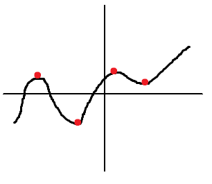
Lagrange is a strategy to find local maxima and minima of a function subject to equality constraints, i.e. max of [latex]f(x,y)[/latex] subject to [latex]g(x,y)=c[/latex]. [latex]f(\cdot)[/latex] and [latex]g(\cdot)[/latex] need to have continuous first partial derivatives.

[latex]\text{ } \quad \wedge (x,y,\lambda) = f(x,y) + \lambda(g(x,y)-c) \quad \lambda \text{ may be positive or negative}[/latex]

If [latex]f(x_0,y_0)[/latex] is a maximum of [latex]f(x,y)[/latex] for the original constrained problem, then there exists [latex]\lambda[/latex] such that [latex](x_0,y_0,\lambda_0)[/latex] is a stationary point for Lagrange function (so [latex]\partial \wedge[/latex] is 0).

In mathematics, a stationary point of a differentiable function of one variable is a point of the function domain where the derivative is zero. For a function of several variables, the stationary point is an input whose all partial derivatives are zero (gradient zero). They correspond to local maxima or minima.

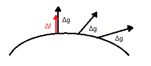
To make it clear, let us say that we have a surface [latex]g(x,y,z)[/latex] whose gradient is [latex]\Delta g[/latex] and it is perpendicular to the whole surface. We try to find its maxima whose gradient should theoretically be perpendicular as well. Let us not forget the relationship between the first derivative and the gradient. Hence we can say that the gradient of [latex]g[/latex] and the gradient of [latex]f[/latex] are pointing in the same direction so: [latex]\overrightarrow{\Delta f} = \lambda \overrightarrow{\Delta g}[/latex] (proportional). [latex]\lambda[/latex] is called Lagrange multiplier.

Example 1: 1 constraint, 2 dimensions

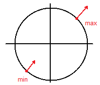
Maximize [latex]f(x,y) = 3x+3y[/latex] on unit circle [latex]x^2+y^2=1 \to g(x,y) = x^2+y^2-1[/latex]

[latex]\frac{\partial f}{\partial x} = \lambda \frac{\partial g}{\partial x} \to 3 = 2x \lambda \to x = \frac{3}{2 \lambda}\\
\frac{\partial f}{\partial y} = \lambda \frac{\partial g}{\partial y} \to 3 = 2y \lambda \to y = \frac{3}{2 \lambda}[/latex]

Now we plug these results into the original equation.

[latex]x^2 + y^2 = 1 \to \frac{9+9}{4 \lambda^2} = \frac{18}{4 \lambda^2} = 1 \to \lambda = \pm \frac{\sqrt{18}}{2} = 2.12 [/latex]

Therefore we have two points:
[latex](x,y) = (0.707,0.707) \quad \text{or} \quad (x,y) = (-0.707,-0.707) \quad \text{so} \quad f(x,y) = 2.12 \quad \text{or} \quad -2.12[/latex]

Example 2: 1 constraint, 2 dimensions

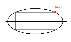
Find the rectangle of maximal perimeter that can be inscribed in the ellipse [latex]x^2+4y^2=4[/latex]. We want to maximize the perimeter which is [latex]f(x,y) = 4x+4y[/latex] subject to [latex]g(x,y) = x^2 +4y^2 -4[/latex]

[latex]\frac{\partial f}{\partial x} = \lambda \frac{\partial g}{\partial x} \to 4 = 2x \lambda \\
\frac{\partial f}{\partial y} = \lambda \frac{\partial g}{\partial y} \to 4 = 8y \lambda \\
x = 4y[/latex]

Now plug it into the original equation.

[latex]x^2+4y^2 = 4 \quad \to \quad 20y^2=4 \quad \to \quad y = \pm \sqrt{\frac{1}{5}}, \quad x=\frac{4}{\sqrt{5}} \quad [/latex] (we take the positive because it is a maximum),

Then, [latex]P = (\frac{4}{\sqrt{5}},\frac{1}{\sqrt{5}})[/latex]
So the maximum permieter is: [latex]f(x,y) = 4x+4y = 4* \frac{4}{\sqrt{5}}+4* \frac{1}{\sqrt{5}} = 4 \sqrt{5}[/latex]

Example 3: 2 constraints, 3 dimensions

[latex]f(x,y,z) = x^2 + y^2 + z^2 \quad \text{subject to} \quad x+y+z=1 \to g_1(x,y,z) = x+y+z-1 \\
\text{ } \hspace{140pt} \text{and } x+2y+3z = 6 \to g_2(x,y,z) = x+2y+3z-6 \\
\vspace{15pt} \\
[/latex]
[latex]
\frac{\partial f}{\partial x} = \lambda_1 \frac{\partial g_1}{\partial x} + \lambda_2 \frac{\partial g_2}{\partial x} \quad \to \quad 2x = \lambda_1 + \lambda_2 \quad \to \quad x = \frac{\lambda_1 + \lambda_2}{2}\\
\frac{\partial f}{\partial y} = \lambda_1 \frac{\partial g_1}{\partial y} + \lambda_2 \frac{\partial g_2}{\partial y} \quad \to \quad 2y = \lambda_1 + 2 \lambda_2 \quad \to \quad y = \frac{\lambda_1 + 2 \lambda_2}{2}\\
\frac{\partial f}{\partial z} = \lambda_1 \frac{\partial g_1}{\partial z} + \lambda_2 \frac{\partial g_2}{\partial z} \quad \to \quad 2z = \lambda_1 + 3 \lambda_2 \quad \to \quad z = \frac{\lambda_1 + 3 \lambda_2}{2}\\[/latex]

Now plug it into [latex]g_1(x,y,z)[/latex] and [latex]g_2(x,y,z)[/latex]:

[latex]\frac{\lambda_1 + \lambda_2}{2} + \frac{\lambda_1 + 2 \lambda_2}{2} + \frac{\lambda_1 + 3 \lambda_2}{2} = 1 \quad \to \quad 3 \lambda_1 + 6 \lambda_2 = 2 \\
\frac{\lambda_1 + \lambda_2}{2} + \lambda_1 + 2 \lambda_2 + \frac{3}{2} (\lambda_1 + 3 \lambda_2) = 6 \quad \to \quad 6 \lambda_1 + 14 \lambda_2 = 12 \\
\lambda_2 = -4, \quad \lambda_1 = \frac{-22}{3} \\
x = \frac{-5}{3}, \quad y = \frac{1}{3}, \quad z = \frac{7}{3} \\
f(x,y,z) = x^2 + y^2 + z^2 \quad f(\frac{-5}{3}, \frac{1}{3}, \frac{7}{3}) = \frac{25}{3}
[/latex]

Since this is a parabola in 3 dimensions, this has no maximum, so it is a minimum.