Laplacian
First order detection is based on the differentiation of intensity within the same region to detect changes whereas the second order gets zero when the rate of change is constant. Therefore, when a zero-crossing is found, the algorithm would have found an edge.
Laplacian operator is a template which implements this. By differentiating between two adjacent pixels (first order), the second order is approximated.
[latex]f”(x) \cong f'(x) – f'(x+1) \\
f”(x) \cong -f(x) + 2f(x+1) -f(x+2)[/latex]
Which can be translated into an horizontal (or vertical if transposed) as:
| -1 | 2 | 1 |
And:
|
|
Marr-Hildreth operator
The Marr-Hildreth operator combines Gaussian filtering to smooth the image with Laplacian (LoG operator, Laplacian of Gauss). After the second differentiation of Gauss we have the corresponding formula to find the coefficients to the template to convolve the image with.
[latex size=”2″]\Delta^2g(x,y) = \frac{1}{\sigma^2}(\frac{(x^2+y^2)}{\sigma^2}-2)e^{\frac{-(x^2+y^2)}{2 \sigma^2}}[/latex]
This function, which can be approximated by a difference of Gaussians, is called Mexican hat wavelet because of its shape:
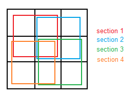
After the image is convolved with the generated template, we have do determine the zero-crossing points. There are many techniques to achieve this goal, but a much simpler solution is shown: first we divide a 3×3 window in 4 sections as in the following picture, all of them containing the pixel in the center. The average of each section is computed, and if the maximum value is positive and the minimum is negative, a zero-crossing is found and therefore the pixel in the center will be set as white (otherwise is marked as black). This has to be applied to the whole image.
Results
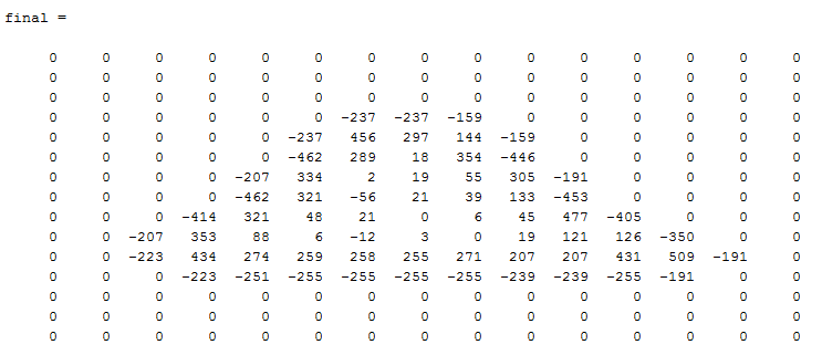
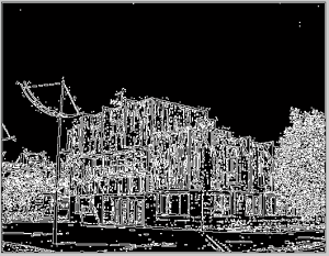
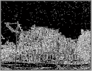
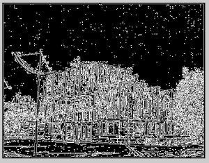
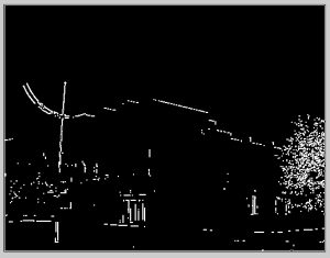
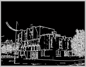
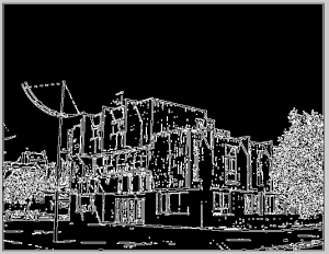
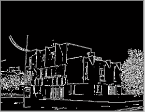
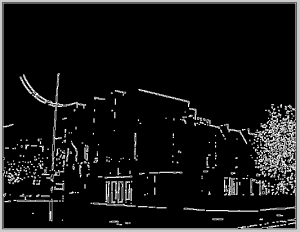
See how a simple figure changes after Laplacian is applied.
Laplacian
In this case we would have to detect the zero-crossings to obtain the final result.
Marr-Hildreth
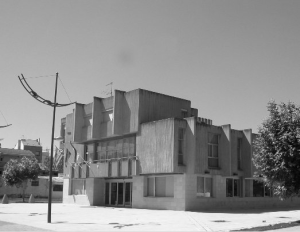
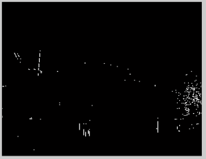
The code is provided in the Source code section.
References
1. M. Nixon and A. Aguado. 2008. “First order edge detection operators”, Feature Extraction & Image Processing.



One thought to “[Second order edge detection operators] Laplacian and Marr-Hildreth operator”