In the previous post I talked about an SVM implementation in Matlab. I consider that post and implementation really interesting since it is not easy to find a simple SVM implementation. Instead, I found tons of files which may implement a very interesting algorithm but they are insanely difficult to examine in order to learn about how it works. This is the main reason why I put so much effort on this implementation I developed thanks to the algorithm [1].
First improvement
After I implemented that algorithm everything seemed to work:
Example 1:

Data points coordinates and target:
Distance to the border from each point: |

Very acceptable results, right? However, when I added more points I experienced an odd behavior.
Example 2:
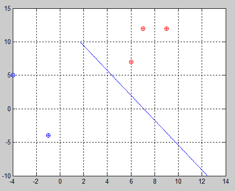

|

It clearly fails at finding the optimum boundary, however, the funny thing here is that the distance between the second and third point and the boundary are the same. This means that the rest of the samples were ignored and the algorithm focused only on those two. Actually, 

After debugging the code everything seemed to be right according to the algorithm I followed [1] but after many trials I saw what definitely brought me to discover the error. In my trial the first two elements belong to class -1 whereas the rest of them belong to the other one. As you can see in the following examples, when I changed the order of the elements in the second class I got that the boundary was different depending only on the first element of the second class, ergo, the third sample.
Example 3:
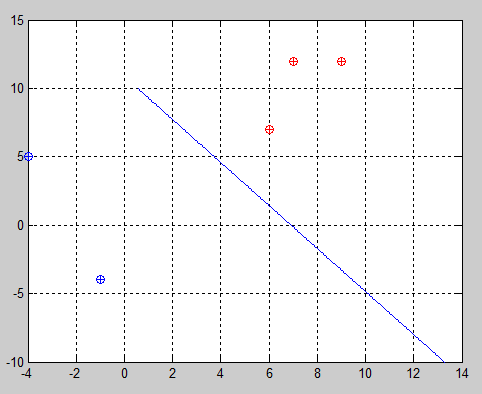

|

Example 4:
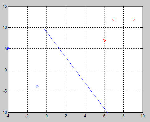

|

In this last trial we get the best solution because in this case the algorithm has to focus on the third sample which is the closest one to the other class. However, this is not always true, so I had the need of fixing it. The fix is very simple but was not easy to find (at least quickly).
When I was debugging the code, I realized that in the first loop (iterating over 
If the samples were not encountered on the 


Thus, the fix in the Matlab code was pretty simple: changing from “break” to “continue“. Break allows to stop iterating over the loop and therefore it continues in the outer loop whereas continue makes the current loop stop and start iterating over the next value in that loop.
Second improvement
After the first improvement was implemented, it seemed that it worked for many trials, but when I tried more complex examples, it failed again.
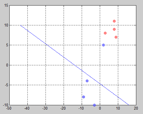

|
The original algorithm [1] uses the variable 

When the algorithm iterates once, alphas are updated such that nonzero alphas correspond to the samples that will help building the boundary. In this example, after the first iteration, alpha values correspond to this:

Therefore, in the next iteration it will update the samples to focus only in sample #3 and sample #6. After this implementation was done, all the trials I tried worked perfectly. This is the result of the same problem:

Algorithm
This is the algorithm [1] after both improvements:
Initialize
Initialize
Calculate 


![\text{while} ((\exists x \in \alpha | x = 0 ) \text{ } \& \& \text{ } (\text{counter} < \text{max\_iter})) [/latex] <span style="margin-left:20px">Initialize input and [latex]\alpha](https://s0.wp.com/latex.php?latex=%5Ctext%7Bwhile%7D+%28%28%5Cexists+x+%5Cin+%5Calpha+%7C+x+%3D+0+%29+%5Ctext%7B+%7D+%5C%26+%5C%26+%5Ctext%7B+%7D+%28%5Ctext%7Bcounter%7D+%3C+%5Ctext%7Bmax%5C_iter%7D%29%29+%26%2391%3B%2Flatex%26%2393%3B+%3Cspan+style%3D%22margin-left%3A20px%22%3EInitialize+input+and+%5Blatex%5D%5Calpha&bg=ffffff&fg=000&s=0&c=20201002)


Calculate 
Save old 
Compute 

Continue to
Compute 
Continue to
Compute and clip new value for 
Determine value for 
Compute 

Compute 


![\text{if } (| \alpha_j - \alpha_j^{(old)} < 10^{-5})[/latex] <b>(*A*)</b></span><br /> <span style="margin-left:100px">Continue to [latex]\text{next j}](https://s0.wp.com/latex.php?latex=%5Ctext%7Bif+%7D+%28%7C+%5Calpha_j+-+%5Calpha_j%5E%7B%28old%29%7D+%3C+10%5E%7B-5%7D%29%26%2391%3B%2Flatex%26%2393%3B+%3Cb%3E%28%2AA%2A%29%3C%2Fb%3E%3C%2Fspan%3E%3Cbr+%2F%3E+%3Cspan+style%3D%22margin-left%3A100px%22%3EContinue+to+%5Blatex%5D%5Ctext%7Bnext+j%7D&bg=ffffff&fg=000&s=0&c=20201002)


Algorithm Legend
(*A*): If the difference between the new 
(*B*): Useful data are those samples whose
(2):
(10):
(11):
(12):
(14):
(15): 
\alpha_j \quad \text{if } L \leq \alpha_j \leq H \\
L \quad \text{if } \alpha_j < L \end{cases}[/latex]
(16): [latex]\alpha_i := \alpha_i + y^{(i)} y^{(j)} (\alpha_j^{(old)} - \alpha_j)[/latex]
(17): [latex]b_1 = b - E_i - y^{(i)} (\alpha_i^{(old)} - \alpha_i) \langle x^{(i)},x^{(i)} \rangle - y^{(j)} (\alpha_j^{(old)} - \alpha_j) \langle x^{(i)},x^{(j)} \rangle[/latex]
(18): [latex]b_2 = b - E_j - y^{(i)} (\alpha_i^{(old)} - \alpha_i) \langle x^{(i)},x^{(j)} \rangle - y^{(j)} (\alpha_j^{(old)} - \alpha_j) \langle x^{(j)},x^{(j)} \rangle[/latex]
(19): [latex]\alpha_j := \begin{cases} b_1 \quad \quad \text{if } 0 < \alpha_i < C \\
b_2 \quad \quad \text{if } 0 < \alpha_j < C \\
(b_1 + b_2)/2 \quad \text{otherwise} \end{cases}[/latex]
The code is provided in the Source code section.


References
1. The Simplified SMO Algorithm http://cs229.stanford.edu/materials/smo.pdf
Hi Juan,
Your blog is really informative and well-written.
I’ve had a look through and downloaded your source code. However, it appears your SVM plotting scripts are not plotting as per the example in this page.
Any chance you could update your github repo?
Cheers
Thank you very much!
I will write a note in my TODO list and I will send you an email. Now I’m on vacations and I will be available next week. I hope I haven’t deleted those files from my other computer 🙂
Regards,
JM.