Image Processing – Lipman’s Artificial Intelligence Directory

Multivariate Gaussian distribution clustering with Expectation Maximization in Python

October 27, 2018October 27, 2018 Juan Miguel Valverde Leave a comment

Expectation Maximization (EM) is a classical algorithm in ML for data clustering. Its theoretical background is based on Bayes theorem and although it’s quite straightforward to follow it might be a bit confusing to implement it in more than 1 dimension.

If you want to understand more about EM I recommend you to check out this and this videos.

EM in a nutshell:

Randomly initialize a mean and variance per class.
Calculate the probability of each data point to belong to those distributions.
Calculate the mean and variance based on those probabilities.
Go to 2. and repeat until convergence.

In the Figure above we can see the initial clusters (top-left), and how the classification is changing in different iterations.

This method considerably relies on the mean and variance initialization. An unlucky initialization will provide with a deficient segmentation.

The code is provided in the Source code section.

Otsu’s method, Python implementation

October 27, 2018October 27, 2018 Juan Miguel Valverde Leave a comment

Otsu’s method is a very old but still used adaptive segmentation algorithm due to its simplicity.

Segmenting an image by setting a threshold is probably the easiest possible approach, but that threshold needs to be established somehow. Otsu’s method looks at the histogram and tries to minimize the within-class variance. In other words, it tries to find a threshold such that the variance of the resulting both classes in the Gaussian distributions is as small as possible.

In the picture above we can guess that a good threshold might be somewhere in between those two Gaussian-like distributions. If you want to learn more about Otsu’s method, check this video.

The code is provided in the Source code section.

Image style transfer using convolutional neural networks – Tensorflow implementation

April 24, 2018April 24, 2018 Juan Miguel Valverde Leave a comment

Recently I recorded a video explaining in a very simple way how style transfer works in a convolutional neural network (VGG16) based on the incredibly well-written paper by Gatys et al [1]. I also implemented it in an extremely concise and simple way (around than 150 lines with comments).

Original Image

Combinations

The code is provided in the Source code section.

References

1. Gatys LA, Ecker AS and Bethge M. 2016. Image Style Transfer Using Convolutional Neural Network.

Homography estimation explanation and python implementation

August 8, 2017August 9, 2017 Juan Miguel Valverde Leave a comment

Homographies are transformations of images from one planar surface to another (image registration). Homographies are used for tasks such as camera calibrations, 3D reconstruction, image rectifications. There are multiple methods to calculate an homography and this post explains one of the simplest.

Given a point in a 3D space [latex]x=(x_1,y_1,1)[/latex] and a matrix H, the resulting multiplication will return the new location of that point [latex]x’ = (x_2,y_2,1)[/latex] such that:

[latex]x’ = Hx[/latex]

Due to the dimensions of [latex]x[/latex] and [latex]x'[/latex] we know that H will be a 3×3 matrix but even if there are 9 elements in the matrix, we will have just 8 degrees of freedom. In this Powerpoint presentation [1] we can intuitively see where does it come from.

So we have that:

[latex]
\begin{bmatrix}
u \\
v \\
1
\end{bmatrix}
=
\begin{bmatrix}
h_1 & h_2 & h_3 \\
h_4 & h_5 & h_6 \\
h_7 & h_8 & h_9
\end{bmatrix}
\begin{bmatrix}
x \\
y \\
1
\end{bmatrix}
[/latex]

Where [latex]u[/latex] and [latex]v[/latex] are the new coordinates. Therefore, we have:

[latex]
\\
u = x h_1 + y h_2 + h_3 \\
v = x h_4 + y h_5 + h_6 \\
1 = x h_7 + y h_8 + h_9 \\
[/latex]

So for each point we have:

[latex]
\\
x h_1 + y h_2 + h_3 – u (x h_7 + y h_8 + h_9) = 0 \\
x h_4 + y h_5 + h_6 – v (x h_7 + y h_8 + h_9) = 0 \\

A_i =
\begin{bmatrix}
x & y & 1 & 0 & 0 & 0 & -ux & -vy & -u \\
0 & 0 & 0 & x & y & 1 & -ux & -vy & -u
\end{bmatrix}
[/latex]

Since we have 8 degrees of freedom, we need at least 4 points to obtain H (each point contributes with two new variables to the formula, x and y). We just need to stack [latex]A_1, A_2, A_3, A_4[/latex] to have a 8×9 matrix that we will call A. We are interested in solving the following equation avoiding the trivial solution h=0

[latex]
Ah=0;
\begin{bmatrix}
x_1 & y_1 & 1 & 0 & 0 & 0 & -u_1 x_1 & -v_1 y_1 & -u_1 \\
0 & 0 & 0 & x_1 & y_1 & 1 & -u_1 x_1 & -v_1 y_1 & -u_1 \\
& & & & \cdots
\end{bmatrix}
\begin{bmatrix}
h1 \\ h2 \\ h3 \\ \vdots
\end{bmatrix}
= 0
[/latex]

We will solve this as a least squares problem using singular value decomposition (SVD)

Least squares and SVD

This method (explained very clearly in [2]) is used when we want to approximate a function given different observations. For instance, we have that:

[latex]
\\
c + d x_1 = y_1 \\
c + d x_2 = y_2 \\
c + d x_3 = y_3
[/latex]

If there were no errors those equations would be true, but since our measurements might have noise we want to minimize that errors by minimizing:

[latex]
(c + d x_1 – y_1)^2 + (c + d x_2 – y_2)^2 + (c + d x_3 – y_3)^2
[/latex]

In general, for systems like [latex]Ax=b[/latex] we want to minimize [latex]|| Ax-b ||^2[/latex]

We will use SVD in our matrix A:

[latex]
[U,S,V] = SVD(A)
[/latex]

V are the eigenvectors of [latex]A^T A[/latex]. The solution is therefore the last eigenvector because its eigenvalue (diagonal matrix D) will be zero or close to zero in case of noise. More intuitively, imagine that the largest eigenvectors will depict the largest variance across the data, and we are interested in minimizing, so the eigenvector should have a small eigenvalue.

When performing an homography, the resulting image will probably have different dimensions from the original one since it might be stretched, rotated, and so on. This will result in having many “empty pixels” that must be filled by performing an interpolation.

One of the nicest properties of the homography is that H has an inverse, which means that we can map all points back to the origin by multiplying them to the inverse of H. In order to fill an empty point we will multiply their coordinates by [latex]H^{-1}[/latex] to get the original coordinates, which will be floating point numbers. Those “original coordinates” must be interpolated (for instance, you can round them) to get the closest pixel (nearest neighbor) and put it in the empty pixel.

Example

In the following example the label of this small notebook will be placed horizontally. For this, the location of the 4 pixels corresponding to the four corners is used, and a new location drawing a rectangle is calculated as well. The red dots correspond to the points we want to transform and the green dots their target location.

This first approximation is obtained by calculating the new location of each pixel. However, it will leave plenty of empty pixels that can be interpolated after the inverse matrix of the homography transformation matrix is calculated.

After the interpolation, the final result will not contain any empty pixel.

The code is provided in the Source code section.

References

1. https://courses.cs.washington.edu/courses/csep576/11sp/pdf/Transformations.pdf (Accessed on 8-8-2017)
2. http://www.sci.utah.edu/~gerig/CS6640-F2012/Materials/pseudoinverse-cis61009sl10.pdf (Accessed on 8-8-2017)

[Explanation] Face Recognition using Eigenfaces

October 5, 2015October 5, 2015 Juan Miguel Valverde 4 Comments

This post comes from an assignment for my “Cognitive Science I” course. Enjoy it.

Brief Introduction

This paper is one of the most relevant papers regarding to face recognition. Nowadays it is difficult to find a real life implementation of this old algorithm, but other research has been built upon this. In addition, the simplistic and effectiveness of this algorithm makes it very beautiful.

Algorithm

To train the model:
1.-Flat the black and white images of the training set (from matrices to vectors)
2.-Calculate the mean.
3.-Normalize the training set: for each image, subtract the mean.
4.-Calculate the covariance: multiply all images by themselves.
5.-Extract eigenvectors from the covariance.
6.-Calculate eigenfaces: eigenvectors x normalized pictures.
7.-Choose the most significant eigenfaces.
8.-Calculate weights: chosen eigenfaces x normalized pictures.

To detect a face:
9.-Vectorize and normalize this picture: subtract the calculated mean from the picture.
10.-Calculate the weights: multiply the eigenfaces x normalized picture.
11.-Interpret the distance of this weight vector in the face space: if it is far, it is not a face (establishment of a threshold).

Explanation of the algorithm

Training set used:

1.-Flatting the image
This algorithm works with vectors because we have to calculate later the covariance. Because of this, the image needs to be in a vector form.

1	2	3
4	5	6
7	8	9

2.-Calculate the mean
The mean is just the sum of all of the pictures divided by the number of pictures. As a result, we will have an “average” face.

3.-Normalize the training set
To normalize the training set, we just simply need to subtract for each picture in the training set the mean that was calculated in the previous step.

The reason why this is necessary is because we want to create a system that is able to represent any face. Therefore, we calculated the elements that all faces have in common (the mean). If we extract this average from the pictures, the features that distinguish each picture from the rest of the set are visible.

4.-Calculate the covariance
The covariance represents how two variables change together. After the previous step, we have a set of images that have different features, so now we want to see how these features for each individual picture change in relation to the rest of the pictures.

For this purpose, we put all the flat normalized pictures together in a vector. My training set consists of 16 pictures whose dimensions are 235×235 pixels. Therefore, the resulting matrix will be 55225×16. The covariance is the multiplication of this matrix by itself, and if we transpose it correctly, the resulting matrix will be 16×16:

16x55225 * 55225x16 = 16×16

5.-Extract eigenvectors
From the covariance we can extract the eigenvectors. Fortunately, there is Matlab function that helps us in this step (you can see it on the code). There is plenty of information in the internet about eigenvectors (2) (3) but the general idea is that eigenvectors are the vectors of the covariance that describe the direction of the data. The first eigenvector will describe more information than the second and so on. For this reason, later we have to pick the first eigenvectors generated (avoiding noise).

6.-Calculate eigenfaces
Each eigenvector is multiplied by the whole normalized training set matrix (the 55225×16 matrix) and as a result, we will have the same amount of eigenfaces as images in our training set.

7.-Choose the most significant eigenfaces.
The first eigenfaces represent more information than the last eigenfaces. Actually, the last eigenfaces only add noise to the model, so it is necessary to avoid them. Therefore, only the most significant eigenfaces are chosen. For this, there are many heuristic algorithms but it can also be done by looking at the pictures. In my code I only used 16 different pictures, and since the training set is tiny, all of the eigenfaces represent important features.

Some simple heuristic algorithms are shown in the code but they are not used. I preferred to manually select the amount of eigenfaces to see the difference in the algorithm’s performance.

Among these heuristics are:
1) To select those eigenvectors whose eigenvalues are above 1.
2) To choose all eigenvectors until the cumulative sum of the eigenvalues is around 95%

8.-Calculate weights
Each normalized face in the training set multiplies each eigenface. Consequently, there will be N set of weights with M elements (N = amount of pictures in the training set, M = number of eigenfaces).

After this procedure, we can theoretically represent each face as a linear combination of the chosen eigenfaces. This means that each picture in the training set can be recalculated by a sum of each eigenface multiplied by the corresponding weight plus the mean.

Recognition part: 9.-Vectorize and normalize the picture
Reshape the test picture into a vector and subtract the mean calculated in 2) from it.

Recognition part: 10.-Calculate the weights
The same as 8) but with the test picture.

Recognition part: 11.-Interpret the distance
Now we have all the weights from our training set and the weight of the picture that we want to classify. The final step is to determine whether the picture is a face or not, given the distance. This can be a bit confusing: the most obvious approach might be calculate the mean of the distances and if the distance is over a predetermined threshold, the picture will be categorized as a face. Nonetheless, this might lead to errors when using, for example, one of the faces used in the training set.

Since the model was trained using the same image, for the system should be obvious to categorize this picture as a face. Unfortunately, that is not the case. The reason is because the distance of the picture used in the training regarding to the specific eigenface that describes its features might be 0 (because it is exactly the same picture) but the distances between this picture and the rest of the images in the training set might be greater, and if we take the mean of the distances, the overall result could be over the threshold that we determined.

The code is provided in the Source code section.
You can also access to the slides of the presentation.

References

1. Matthew A. Turk & Alex P. Pentland. 1991. “Face recognition using Eigenfaces”.
2. “Principal Component Analysis 4 Dummies: Eigenvectors, Eigenvalues and Dimension Reduction”. https://georgemdallas.wordpress.com/2013/10/30/principal-component-analysis-4-dummies-eigenvectors-eigenvalues-and-dimension-reduction/ (Accessed 5-10-2015)
3. Eigenvectors and Eigenvalues Explained Visually. http://setosa.io/ev/eigenvectors-and-eigenvalues/ (Accessed 5-10-2015)

[Hough Transform] Ellipse detection and space reduction

June 23, 2015June 23, 2015 Juan Miguel Valverde 1 Comment

This is the last entry regarding Hough Transform. I previously wrote about Line Detection and Circle Detection including some Source Code, but in this case I will just write about it. The reason why I did not write any code is because it can be found in [1] and because it is very similar to the Circle Detector.

Brief Introduction

Ellipse detection is another useful tool that may have various applications in the field of recognition. Let us not forget that sometimes due to the movement when a picture is taken, in some images circles cannot be represented correctly, so ellipses appear instead. Ellipses are also a very simple shape that can be interesting to recognize since we live surrounded by objects with that shape. As an example, self-driving cars are intended to recognize traffic signs. In particular, rounded traffic signs may look elliptical when they are seen from a specific point of view.

Simple way (5 dimensions)

This approach is very similar to the Circle Detector. Circumferences have 3 characteristics needed to be defined: radius and center coordinates. Likewise, it can be said that in case of ellipses we need 5 characteristics: the center (2), the size along both axes (2) and its rotation (1).

Implementing a 5 dimensional matrix will lead us to fall over the curse of dimensionality. This approach can be reasonable when the algorithm faces a known environment and therefore some characteristics can be drastically reduced. For instance, if a fixed camera aims to capture the movement of the moon, the size of its radius will not change very much, and as the movement can also be predicted, one can simply modify a few parameters to adapt the algorithm and focus on a certain region.

The implementation, as stated above, is similar to the circle detector: using the trigonometric characteristics of the ellipse one can establish relationships between them and iterate over each parameter to try all combinations along the whole image. There is a Matlab code written in [1] (page 209).

Space Reduction

Space reduction is applied in a very similar way to the Circle Detector. Nonetheless, as ellipses are figures a bit more complex than circumferences, it can be more problematic to achieve the solution. Let us recall that for circumferences, it is only necessary to take the center point in the chord between two prospective points that might belong to the circumference, and draw a perpendicular line to the chord passing through the center point. This is possible due to the orthogonality between these two lines, but this is not the case when analyzing ellipses. The equivalent to that perpendicular line in the circumference must be found in other way, for instance, using the tangential lines of those two chosen points, as we can see below.


Circle detection		Ellipse detection

The algorithm shown in the book [1] is similar to the Circle detector: it iterates over the whole picture trying to find a black pixel. When it is detected, it looks in the neighborhood for another one to draw a chord and therefore, the pixel in the center of the chord. The proposed way to find the coordinates of the pixel out of the ellipse is by the intersection of the tangent of those two chosen points. The author proposed that these tangents can be obtained before the process of Non-Maximum Suppression. In this case, during the use of Sobel filter the angles to generate those tangents can be obtained when Canny Edge detector is used.

Finally, we just need to obtain the maxima of the accumulator, and draw the consequent ellipse.

References

1. M. Nixon and A. Aguado. 2008. “First order edge detection operators”, Feature Extraction & Image Processing.

[Hough Transform] Circle detection and space reduction

June 22, 2015June 22, 2015 Juan Miguel Valverde 1 Comment

Brief Introduction

Hough Transform was already used for Line detection and it showed how powerful it can be. This time, the main goal will be detecting circles. Detecting this basic shape may be interesting in the field of recognition since many objects subject to be classified have a circular shape such as the iris of the eyes, coins or even cells under a microscope.

Simple way (3 dimensional matrix)

This first method is easier to understand but very inefficient compared to the next (after space reduction is applied). A circle needs three parameters: x,y values for the center location and the radius of the circumference. Thus the accumulator matrix will have 3 dimensions, one for each parameter, covering all possibilities.

Given a certain radius, when a pixel is detected, the algorithm will increment the accumulator elements corresponding to the circumference that can be drawn using that pixel and radius as characteristics of the circle.

The first two parameters of the 3-D accumulator are x,y values corresponding to the coordinates of the whole picture. The third parameter is the radius. In the following picture, we are using a fixed radius to make everything easier to understand, and the accumulator is incremented in those coordinates in which a red pixel is located.

As you can see, the red pixels almost do not coincide in any point when iterating over the same coordinate. During the algorithm execution, many circles will be drawn and there will be a peak in the center of the real circle we want to detect, as depicted below. They all meet in the center of the circumference (green points).

When the algorithm finishes the iteration over all pixels and radius, we only need to find where is that maxima located to get the characteristics of the circumference. Finally, we can draw it.

The most problematic characteristic of this algorithm is that it needs to iterate over all radius, so it will lose a considerable amount of time on this task. For this reason, in the algorithm I developed I establish a min and max radius, to avoid checking radius extremely short and radius too large. This is how it looks depending on the described situation.


a)		b)		c)

a) When the circumference has a larger radius than expected.
b) When it finds more figures.
c) When it only finds an ellipse.

The algorithm is this:
Iterate over columns (x)
Iterate over rows (y)
If an edge is detected
Iterate over all radius (r)
For angles between 0 and 360 (m)
Calculate pixel for the generated circumference (y,x,r)
If that pixel is not out of bounds, increase accumulator

Space Reduction

Space reduction in this case consist in removing the problematic radius parameter.

When iterating over the picture and a pixel is detected, it will try to look for more pixels in a enclosed neighborhood. When a pixel in the neighborhood is detected, we will have an arc of the circumference. Given these two pixels, we will have a slope and a middle point (blue). We need to find the perpendicular line passing through that middle point (red) which represents the increment in the accumulator.

As the algorithm iterates, it will increase more and more the accumulator, and a peak in the center of the real circumference will be generated.


After some iterations		Accumulator plotted

There is another method to obtain the center explained in [1], but the algorithm written in the book is an implementation of the already explained method. However, the author of the books does not give a hint about getting the radius once we got the center.

I used a 1 dimensional array (or vector) as an accumulator of the distances of each pixel in the image to the center. The peak will be generated when the distances of all the pixels belonging to the circumference are summed in the accumulator. This results in the radius of that circumference. It may be improved by starting in the neighborhood of the center and stop counting at some point.

The execution time differs from the improved algorithm and from the non-improved algorithm. For the same picture, the non-improved algorithm takes around 0.39 seconds whereas the improved version takes around 0.019 seconds.

The code is provided in the Source code section.

References

1. M. Nixon and A. Aguado. 2008. “First order edge detection operators”, Feature Extraction & Image Processing.

[High and low pass filters] The Einstein-Monroe picture

June 22, 2015August 8, 2017 Juan Miguel Valverde 3 Comments

There is an Einstein-Monroe picture wandering around the Internet that I recently saw. It can be a nice example of how human vision works as well as building a high and low pass filter from scratch in order to extract both images.

This picture includes a low frequency picture of Monroe and a high frequency picture of Einstein blended together. Human vision notices details of its environment when objects are close (high frequency). That means that when we are close enough (a normal distance) to this picture, we should be able to see Einstein’s face, otherwise you should check your sight. If you take 3 steps back and see the same picture, you should be seeing Monroe’s face because your vision is not able anymore to get the small details of the picture. Instead, it will get a general idea of the picture (a bit blurry).

Since this is about high and low frequency pictures, we can build high and low pass filters to extract the frequency of the image we want. Thus each original image is theoretically possible to be extracted.

First of all, we can see how the Fast Fourier transform looks like. In order to achieve it, we have to perform the 2-D Fast Fourier, shift it, and scale it.

The low frequency data of the image is in the center of the previous image. Thus a simply low-pass filter can be built by keeping the center and removing the rest, as this picture shows. If we want to extract the opposite, we can invert it.


Low-pass filter		High-pass filter

The radius of the circle needs to be manually adjusted depending on the output. When we try to rebuilt the image using both of those Fourier Transform, we get the original images.


Low frequency image		High frequency image

Since in my secondary screen I can barely see Einstein’s face, I tried to increase the contrast to make it easier to see in case you have the same issue.

The code is provided in the Source code section.

Interesting Links

1. S. Lehar. “An Intuitive Explanation of Fourier Theory”, http://cns-alumni.bu.edu/~slehar/fourier/fourier.html.

[Hough transform] Line detection (Cartesian, Polar and Space reduction)

June 19, 2015June 19, 2015 Juan Miguel Valverde 4 Comments

Brief Introduction

Line detection is one of the most important and basic feature extraction methods. Many currently developing and promising fields such as self driving cars may use line detection to detect lanes. Thus, it is important to understand how it works (both mathematically and the implementation).

As we are using a 2D plane (an image) we can use Cartesian or Polar parameterization. Polar parameterization is useful not only because of its own advantages, but also because it allows the algorithm to reduce costs by space reduction.

Cartesian

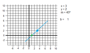
Let us keep in mind the line equation:
[latex]y = mx + c[/latex]
In homogeneous form:
[latex]Ay+Bx +1 = 0 \quad[/latex] where [latex]A = -1/c, B = m/c[/latex]

To determine the line we must find [latex]m, c \quad \text{(or A, B)}[/latex]

The way HT works is by simply counting the potential solution in an accumulator, tracing all possible lines for each point within the main iteration. Hence, finding the maximum in the accumulator means finding the line with the highest probability.

When iterating, after checking that a black pixel (typically corresponding to an edge) has been detected, it iterates over two different “for” loops. The first loop corresponds to angles between -45 and 45 degrees (both inclusive) and the second loop between 45 and 135. It is necessary to separate them because for slopes whose degrees are larger than 45 or lower than -45, [latex]c[/latex] (intersection with y-axis) may take large values. Thus, an additional accumulator for angles between 45 and 135 is needed, which will store a similar [latex]c[/latex] variable whose value is the intersection with x-axis rather than y-axis.

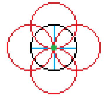
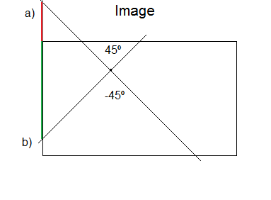
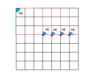
As we can see in the image below for the case when angles are between -45 and 45, when [latex]c[/latex] is out of bounds (a) (bounds are 0 and the height), the accumulator is not increased. Otherwise, the accumulator will increase for all those angles between the allowed boundaries (b) (green). Note that all those angles that are outside are later taken into account when examining x-axis.

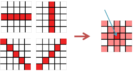
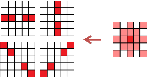
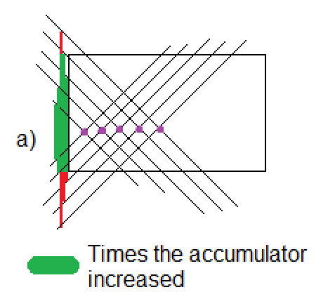
In the following picture, we have 5 points that may compound a line. In the green zone of the left side you can see how the region in the middle is getting larger and larger. That represents the accumulator values for those angles and intersection with the y-axis, and it shows that there is a high probability to find a line, as it is. Likewise, we can also see that the behavior of this algorithm is strong against noise and occlusion. As a drawback, two large matrices are needed.

Cartesian Algorithm

Iterate over rows (y)
Iterate over columns(x)
If an edge is detected
For angles between -45 and 45 (m)
Calculate c (y-axis intersections)
If c is between the bounds, increase accumulatorA
For angles between 45 and 135 (m)
Calculate c (x-axis intersections)
If c is between the bounds, increase accumulatorB

Cartesian Examples

Correction

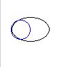
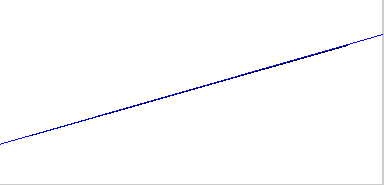
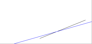
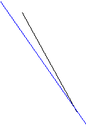
The previous algorithm taken from [1] was used to understand Hough Transform for Cartesian coordinate systems, however, this algorithm failed to classify some lines such as the following:

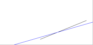
At first I thought that the problem could be my implementation of how to draw those lines given the accumulators, but after a deep study of the algorithm I realized what was the mistake. In addition to the author mistake, I added a small improvement that may help to understand HT in Cartesian coordinate systems.

First of all, in the author’s algorithm the accumulators are split depending on the degrees that are being examined. The first accumulator stores vertical intersections of the y-axis on angles between -45 and 45 whereas the second is responsible of the x-axis intersections on angles between 45 and 135.

If a nearly horizontal line is examined, the first accumulator (vertical intersections) will have a higher maxima than the second accumulator. This can be seen in the image above the algorithm: in the vertical accumulator a peak around the center will be created. In contrast, the horizontal accumulator will grow but very plain. Let us recall that in the accumulator there are represented the pixel where the line should start (the intersection with the axis) and the angle. Once this is completely understood, one can imagine many problematic scenarios such as the one depicted previously.

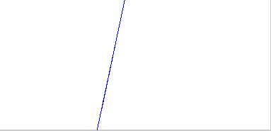
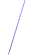
In the previous image, the line that should be generated must start in the x-axis. This means that the horizontal accumulator (the second) should have a higher peak than the vertical one. However, the angle corresponding to that line is between -45 and 45 degrees, so it is only examined by the first accumulator. Thus, the assumption that one accumulator should be in charge of a certain range of degrees while the second takes cares of the rest, is extremely naïve. The solution to this problem is by simply computing the range from -45 to 135 degrees in both accumulators. It is worth saying that the computation time is almost not affected at all, but we need a higher amount of memory.

The improvement to better understand the algorithm is more related with the later line drawing. As the “for” loops and pixel detection works, the image is examined from top to bottom and left to right. This makes our coordinates system move from the typical 0,0 starting in the bottom-left corner to the top-left corner. This shift arises problematic issues regarding the formulas, especially with the one used for the second accumulator (x-axis crossings detection). The formula used for detecting these crossings is:

[latex size=”1.5″]b = \text{round(} x- \frac{y}{\tan{m* \pi / 180}} \text{)}[/latex]

Where [latex]m[/latex] represents the angle and [latex]x, y[/latex] represent the coordinates. This formula may work when the 0,0 is in the bottom-left corner:

But if the coordinate epicenter is moved, it will not work anymore. For this reason, instead of computing [latex]y[/latex] when [latex]b[/latex] is calculated, I decided to compute [latex]yInv = rows – y[/latex]. An alternative solution would be changing the formula.

Final algorithm:
Iterate over rows (y)
Iterate over columns(x)
If an edge is detected
For angles between -45 and 135 (m)
Calculate yInv ([latex]yInv = rows – y[/latex])
Calculate c (y-axis intersections)
If c is between the bounds, increase accumulatorA
Calculate c (x-axis intersections)
If c is between the bounds, increase accumulatorB

Both algorithms (the original and the improved one) are in the Source code section.

Polar

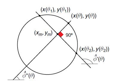
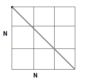
Polar coordinate system is an alternative to the Cartesian in which a radius and angle are needed to locate a single point, rather than X-Y coordinates. The maximum length of the radius can be obtain by the Pythagoras formula: [latex]\sqrt{2} N[/latex] where N is the largest size (width or height).

In contrast with Cartesian, in the Polar algorithm we only need one accumulator. The first dimension of the matrix is the radius which is between 0 and [latex]\sqrt{2} N[/latex], and the second dimension is the angle (0-180). It will work in the same way as Cartesian: examining each point of the edge individually the accumulator will increase in those points which may generate the objective line. The final line will be drawn by finding the maximum value in the accumulator and using the radius and angle where it is located. It may seem a bit confusing how to calculate prospective points in the Polar coordinate system, so I tried to explain it using some drawings.

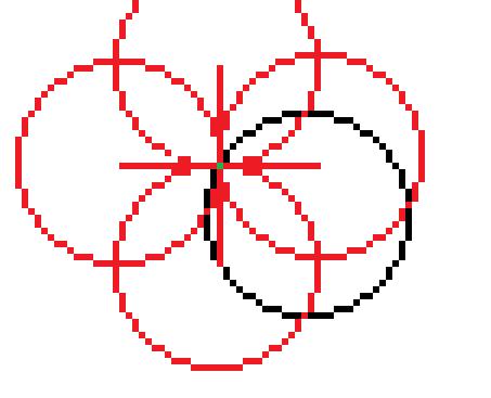
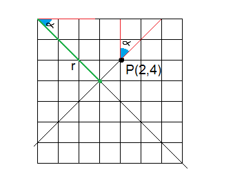
Imagine that we have the point 2,4. It is not difficult to calculate its angle and radius.

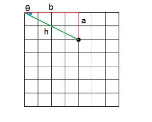
[latex]r = \sqrt{x^2 + y^2} = \sqrt{4^2 + 2^2} = 4.47 \\
\sin{\theta} = \frac{a}{c}; \theta = 26.5[/latex]

However, for the same point, it looks a bit confusing when examining different angles. This is how it looks when we try to figure out the radius of the same point for a 45º angle.

And here is an example of a straight line: 4 purple points in a row. If we examine all the angles, we will realize that for the 90º angle they all reach the same point (3), so the accumulator will be maximum there.

Polar Algorithm

Initialize max value of radius [latex]\sqrt{2} N[/latex]
Iterate over columns (x)
Iterate over rows (y)
If an edge is detected
For angles between 1 and 180 (m)
Calculate the radius (*)
If radius is between the bounds (0 and maximum), increase accumulator

Polar Examples

The same pictures as Cartesian Examples.

Correction

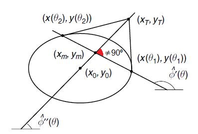
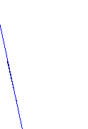
As in the Cartesian algorithm given in [1], in the Polar algorithm another mistake related to the one found in the Cartesian is found as well. This algorithm seems to work always except for one particular case: when one side of the line is bent pointing from top to bottom following a north-west to south-east direction.


Ok.		Fail		Ok.

Again, the error is to naïvely assume that the previous studied radius-angles were all the possibilities.

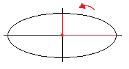
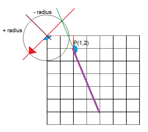
The error is illustrated in the picture below. Given that angle (around 150º) the corresponding radius is negative and therefore, it is discarded (radius must be between 0 and [latex]\sqrt{2} N[/latex]). The reason why the radius is negative is very simple: the intersection is in the other side of the line to which it is suppose to intersect (the red line with the arrow). Given this scenario the solution could be a negative radius and 150º degrees or a positive radius but a negative degrees (150-180 = -30º). Both scenarios cannot be stored in the accumulator for obvious reasons. The real (and more expensive in terms of memory) solution would be to extent the accumulator from 1-180 to 1-360 degrees to cover all cases. In this case, this line would be detected in the angle -30+360 = 330º and the radius will be positive because of the orientation of the arrow.

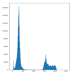
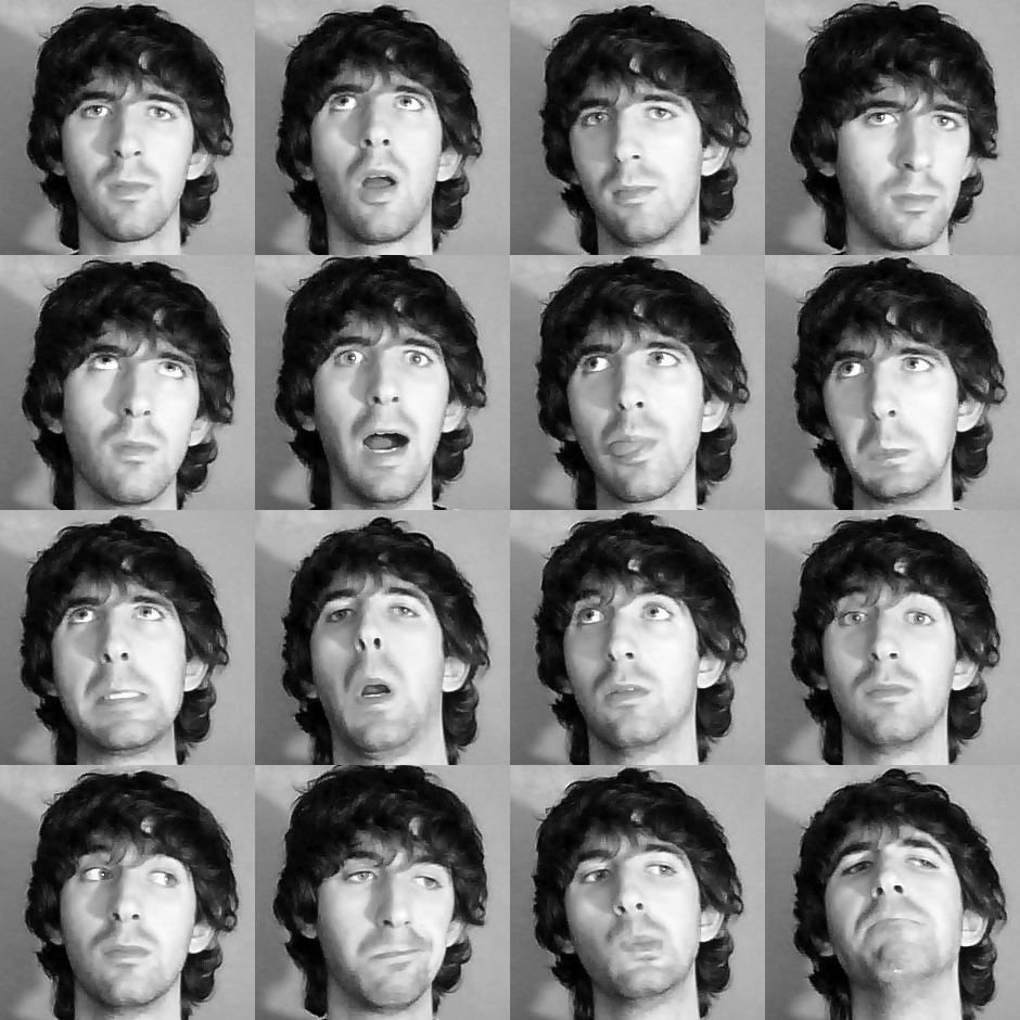
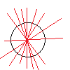
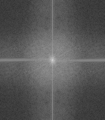
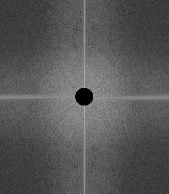
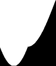
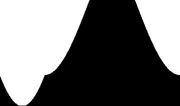
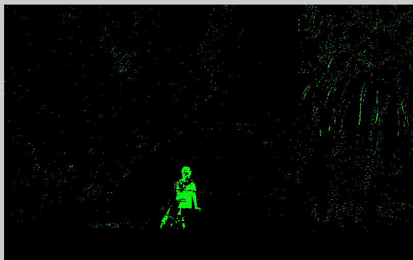
Nonetheless, I tried to study how good or bad was assuming that we only needed to check 1-180 degrees. For this, I run the algorithm through a 150×150 black image to make it fire in every pixel and try each combination. After that, I checked which parts of the accumulator were 0, meaning this that the will never be modified. I did the same in the 1-360 case to see those cases that cannot be seen from the first 1-180º implementation. The black color represents those elements who are never increased whereas the white color represents a zone that can be modified. The width indicates each angle, so in the first case the picture has 180 columns and the second one has 360.

The conclusion drawn from these pictures is that it is possible to make a more efficient algorithm to iterate only over those cases that may be meaningful.

Space Reduction

The space reduction is a modification of the polar algorithm in which the accumulator matrix is reduced from [latex]\text{max},180[/latex] to two matrices: [latex]180,1 \quad \text{and} \quad \text{max},1[/latex]. The huge save is obvious, but again, the naïve approach to enclose the problem from 1 to 180 degrees will have the same consequences as in the previous section.

The algorithm presented in the book does not iterate over all angles. Instead, it checks whether a point is located in a certain neighborhood (a 5×5 window) and it calculates the angle for that point.

This approach is more statistical than the previous algorithms, so instead of the accuracy given by knowing the coordinates which correspond to the characteristics of the line, it decides the parameters of the line given the statistics from the accumulator.

The code given in [1], page 211, does not work for almost any line. To make it work, one needs to fix it as in the previous section: adding the 360 degrees.

Additional notes for further improvements

·The accuracy is extremely related with the counter value
·Instead of taking the max, you can take the 2 or 3 max values since more lines may be found.
·Instead of 2 or 3 max, you can establish a threshold
·It can also be possible to study only those lines in a certain region of the picture. For instance, if you want to make a lane recognizer you should focus on the half in the bottom.

The code is provided in the Source code section.

References

1. M. Nixon and A. Aguado. 2008. “First order edge detection operators”, Feature Extraction & Image Processing.

[Image Processing] Thresholding and Subtracting

June 14, 2015June 22, 2015 Juan Miguel Valverde 1 Comment

One of the simplest methods to extract features from a picture is by subtracting and thresholding. Imagine that from a static background we want to get any figure that appears in front. For instance, let us say that we want to measure the height of different people who will lean against a wall. At first, the background (the wall) is observed. Then, someone will appear, and later, by subtracting the new picture from the background we will be able to extract the person who appeared. After that, it will not be difficult to guess the height. The thresholding operation comes from the fact that we have to decide how strong is the change to consider that it indeed changed.

The most impressive advantage of this method is that it is really easy to implement and fast, similar to the temporal median which can actually be used to generate the background. The biggest drawback is that it is very sensitive to noise and luminosity changes as we will see.

I cropped a couple of pictures used in the temporal median to try this out.

Background

Background + figure

And these are the results after applying thresholding and subtraction. The first picture has a lot of noise as you can see, but I think is very easy to remove in this case. I think this noise comes from that when these pictures were taken, there was a bit of wind and pixels are not exactly the same. In order to remove the noise, in the second attempt I firstly used a Gaussian filter. By the way, both pictures were converted first to gray scale to make it simple and faster since the background and foreground will be in a different color, although Gaussian took really long compared to the first one. In any case, in the original image my right arm is almost blended with the background. That is why it is not well detected.

Simple thresholding and subtracting

Using a Gaussian filter first

When subtracting you can be very imaginative and try different things depending on the background, foreground and the application:
a) Having single thresholds for each color channel
b) Having a global threshold made from the sum of the subtracting of each channel
c) Combining a) and b)
d) Using gray scale
e) Applying a template convolution (Gaussian or any other)
f) Check out the neighborhood
and so on.

I wanted to try out how to use the webcam to process and show the results “in real time”, although my computer does not compute very fast and I took a picture every 1 or 1.5 seconds, but it is still interesting. I also wrote a post about how to take pictures from the webcam with Matlab.

This is the algorithm of the code I made

Initialize webcam, max_times
Wait 2 seconds before taking a picture of the background (to let me hide)
Take a picture of the background
Wait 1 second
while max_times>=0
Take a picture
result = blackPicture (background color)
Iterate over each pixel (y,x)
If background(y,x,redChannel) – picture(y,x,redChannel) > threshold || background(y,x,greenChannel) – picture(y,x,greenChannel) > threshold || background(y,x,blueChannel) – picture(y,x,blueChannel) > threshold
result(x,y,channels) = newColor
End if
Show picture (or store it)
Decrease max_times

Results

Some times we can see that the whole area is green. This is because the luminosity changes depending on where the camera is focusing, and the focus changes depending on where the camera detects something. As the luminosity of the whole picture changes, everything turns to green. Shadows also make the luminosity change.

An example of how luminosity changes depending on where the webcam is focused.

Background picture

Take a look to the luminosity of the walls

The code is provided in the Source code section.

References

1. M. Nixon and A. Aguado. 2008. “First order edge detection operators”, Feature Extraction & Image Processing.