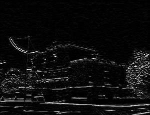
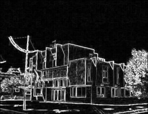
[Edge detection] Canny edge detector

Process of Canny edge detection algorithm

There are three well differentiated steps:
1.-Apply Gaussian filter to remove noise
2.-Apply non-maximum suppression to remove useless edges
3.-Apply hysteresis to add well connected edges

1.-Apply Gaussian filter

Gaussian filter has been explained separately.

2.-Apply non-maximum suppression

The general idea of this process is that after applying a Gaussian filter to remove the noise, we need a tool to detect edge values such as Sobel filter. The value generated by doing the square root of both partial values squared will be denominated intensity from now on. The edges obtained by doing a Sobel filtering have different intensity, and the goal of non-maximum suppression is to keep the highest intensity edge pixels while removing the others, because usually a edge consist of a thin line of pixels rather than many of them.

When Sobel is used during this process, horizontal and vertical templates are:
[latex]
G_x = \begin{bmatrix}
-1 & 0 & +1 \\
-2 & 0 & +2 \\
-1 & 0 & +1
\end{bmatrix}

\quad \text{and} \quad

G_y = \begin{bmatrix}
+1 & +2 & +1 \\
0 & 0 & 0 \\
-1 & -2 & -1
\end{bmatrix}
[/latex]

The reason why I used a slightly different templates than in the Sobel filter entry is explained there.

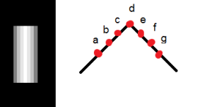
Have a look to this simple edge where intensities are represented using different colors (the whiter, the higher intensity), and imagine that intensity represents the height of each pixel so that we want to remove all except the one in the top of the ridge. We need to find the highest intensity element, and for this task we can look at the direction of each pixel to go upwards.

int1

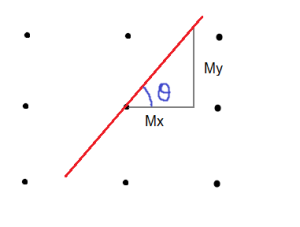
Directions can be obtained by the Gx and Gy values used for calculating the intensity, by simply:

[latex]
\theta = \arctan \frac{G_y}{G_x}
[/latex]

The direction is the vector orientation.

orientation

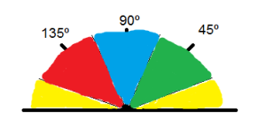
Depending on the angle, directions can be vertical, horizontal, diagonal-left, diagonal-right.

angles

Horizontal: 0 to 22.5 & 157.5 to 180 degrees
Vertical: 67.5 to 112.5 degrees
Diagonal-Left: 112.5 to 157.5
Diagonal-Right: 22.5 to 67.5

Now that for each pixel we have an intensity and direction, note that there can only be 2 more pixels surrounding our pixel in that direction, and we need to compare it with this two pixels. So if we have a pixel which has a vertical direction, it will be compared with the pixels above and below it (if no problem is encountered due to the borders). When comparing it, if a higher value is found, our pixel will be set to zero (black). Otherwise its value will be preserved.

Let us say that I have a simple figure like this, to which I applied Sobel filter. Let us focus on a certain region (the right-bottom corner above the red line).

a1
Figure (20×20)
a2
After Sobel

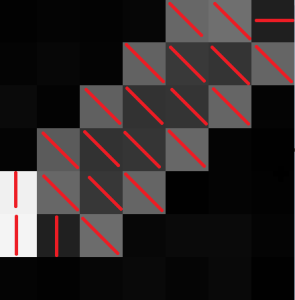
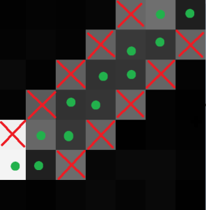
On the first picture I wrote the intensity values whereas on the second one I depicted its orientation. In the last picture we can see which pixels were preserved and which were set to zero.

a31
Intensity
a32
Directions
ares
Result after comparing neighbors

3.-Apply hysteresis

Hysteresis’ process basically aims to threshold the whole image. Nonetheless, it does not use a single threshold, but two instead. We need to understand this as an attempt to extend the threshold giving to the algorithm a higher flexibility. For instance, I may find a pixel which is above the threshold and therefore considered as an edge, but right after it I may find another pixel which is part of the edge but its intensity is slightly below our threshold. That is the reason why the algorithm uses two thresholds.

The algorithm may be as:

Iterate over rows
Iterate over columns
If pixel is above threshold
Make this pixel white
For each surrounding pixel: if it is above the second threshold
Make surrounding pixel white
Else: make surrounding pixel black
Else: make this pixel black

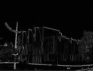
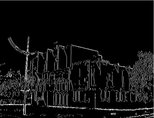
Results (evolution of the process)

Note: Of course that these results may be better. You just need to keep playing with the parameters until you adjust it appropriately.

original
Original
gauss
Gauss: {kernel’s size: 9, sigma: 1}
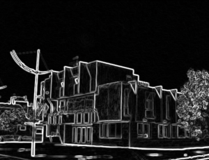
sobel
Sobel: {kernel’s size: 3}
nonmaxsupr
Non-maximum suppression
hyst
Hysteresis: {upperThreshold: 50, lowerThreshold: 30}

The code is provided in the Source code section.

References

1. M. Nixon and A. Aguado. 2008. “First order edge detection operators”, Feature Extraction & Image Processing.
[Edge detection] Sobel Filter

History and Evolution

In order to detect edges, it seems obvious that we need to compare the intensity of adjacent pixels (vertical and horizontal). If the difference is high, we will probably have found an edge.

[latex]
E_x = P_{x,y} – P_{x+1,y} \quad \text{vertical} \\
E_y = P_{x,y} – P_{x,y+1} \quad \text{horizontal}
[/latex]

After we combine them:

[latex]
E_{x,y} = P_{x,y} – P_{x+1,y} + P_{x,y} – P_{x,y+1} \\
E_{x,y} = 2*P_{x,y} – P_{x,y+1} – P_{x+1,y}
[/latex]

Therefore, our coefficients are:

[latex]
K = \begin{bmatrix}
2 & -1\\
-1 & 0
\end{bmatrix}
[/latex]

Trough an Taylor series analysis (you can find the formulas in pages 119 and 120 of the referenced book) we can see that by differencing adjacent points we get an estimate of the first derivative at a point with error [latex]O(\Delta x)[/latex] which is the separation between points. This operation reveals that this error can be reduced by spacing the differenced points by one pixel (averaging tends to reduce noise). This is equivalent to computing the first order difference viewed in the previous formula at two adjacent points, as a new difference where:

[latex]
Exx_{x,y} = Ex_{x+1,y} + Ex_{x,y} \\
Exx_{x,y} = P_{x+1,y} – P_{x,y} + P_{x,y} – P_{x-1,y} \\
Exx_{x,y} = P_{x+1,y} – P_{x-1,y}
[/latex]

Hence:

[latex]
Mx = \begin{bmatrix}
1 & 0 & -1
\end{bmatrix}

\quad

My = \begin{bmatrix}
1 \\
0 \\
-1
\end{bmatrix}
[/latex]

Prewitt edge detection operator extended both templates by adding two additional rows (or columns). This is due to the fact that averaging reduce noise.

[latex]
Mx = \begin{bmatrix}
1 & 0 & -1 \\
1 & 0 & -1 \\
1 & 0 & -1
\end{bmatrix}

\quad

My = \begin{bmatrix}
1 & 1 & 1 \\
0 & 0 & 0 \\
-1 & -1 & -1
\end{bmatrix}
[/latex]

Finally, we can say that the Sobel edge detector is a simple modification of this.

Application

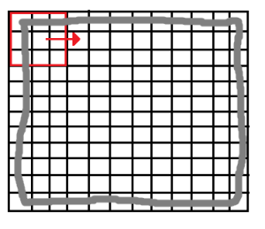
The application of this algorithm is as any other kernel based algorithm. We have two different kernels that need to be applied (convolved) to the image independently. This is done by shifting the kernel through the rows and columns as depicted, and multiplying by each element.

[latex]
G_x = \begin{bmatrix}
-1 & 0 & +1 \\
-2 & 0 & +2 \\
-1 & 0 & +1
\end{bmatrix}

\quad \text{and} \quad

G_y = \begin{bmatrix}
-1 & -2 & -1 \\
0 & 0 & 0 \\
+1 & +2 & +1
\end{bmatrix}
[/latex]

im1

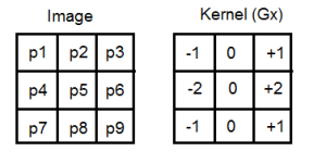
The kernel’s size is odd (typically 3 or 5) so there is no problem fixing it and having a centered valued. During each iteration, we need to multiply each element of the windowed picture with each element of the kernel, and sum it together.

im2

[latex]
V_x = -1*p_1 + 0*p_2 + 1*p_3 + -2*p_4 + 0*p_5 + 2*p_6 -1*p_7 + 0*p_8 + 1*p_9
[/latex]

As I have said previously, during each iteration we need to compute Gx and Gy kernels, so we will end up with two values. The following operation is needed, and its result will be placed in the position of middle of the matrix (P5) in a different matrix which will have the final image:

[latex]
G = \sqrt{G_x^2 + G_y^2}
[/latex]

Note that because of this procedure, borders (2 images below marked with gray) will be lost. The larger is the kernel’s size, the more border will be lost. Nonetheless, this is not usually a problem since our goal is usually located at the center of the image.

In conclusion, the algorithm may be the following:

Iterate over rows
Iterate over columns
Convolve the windowed region with Gx
Convolve the windowed region with Gy
Solve square root
Write that value on the output picture

About Sobel templates

[latex]
G_x = \begin{bmatrix}
-1 & 0 & +1 \\
-2 & 0 & +2 \\
-1 & 0 & +1
\end{bmatrix}

\quad \text{and} \quad

G_y = \begin{bmatrix}
-1 & -2 & -1 \\
0 & 0 & 0 \\
+1 & +2 & +1
\end{bmatrix}
[/latex]

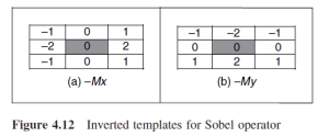
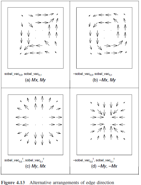
These templates are probably the most used that you can find in the literature about Sobel filter, but you can actually see that when using Sobel filter in Canny edge detector I used a slightly different ones.
This is because Sobel edge direction data can be arranged in different ways without modifying the general idea of the filter. Therefore, depending on the template’s orientation, points will have different directions, as we can see in the following pictures extracted from the book I used.

pic1

pic2

Results

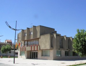
utebo
Original
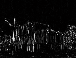
sobelx
Sobel Y-axis
sobely
Sobel X-axis
sobel
Sobel (combined)

The code is provided in the Source code section.

References

1. M. Nixon and A. Aguado. 2008. “First order edge detection operators”, Feature Extraction & Image Processing.