Recently I was reading about Monte Carlo and I decided that I had to implement one of its versions before going further to the next chapter in order to fully understand it. Personally Monte Carlo was a bit hard to understand because it’s not a simply algorithm or bunch of algorithms, but a general framework of solving problems instead. Finally, after reading the corresponding chapter [1] I went down to work and started to think and design a toy problem in Matlab.
Matlab design explanation
The most interesting thing is that I developed it very generically: you can set the start and goal state and generate a customized configuration of the walls (or randomized, or no walls at all). It only have the condition that you can only use 36 states, which I considered enough for a simulation.
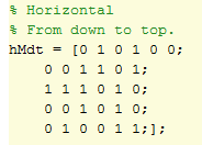
I faced two problems when developing this algorithm. The first one made me lose roughly one hour since I was using relative values to draw the elements, but I finally changed to pixels because I can have an exhaustive and exact control about the size of each square. The second problem was the orientation. My mind was quite messed up thinking what should be better. The choices were: being the (1,1) element the square in the left-bottom corner (as it’s usually in the graphs that I’m used to), being the (1,1) element the square in the left-top corner (easier to deal with matrices in Matlab), and in this last case, should the first element of the matrix be the vertical distance (as it’s in the matrices in Matlab) or should I follow my intuition with the graphs? At the end, I decided to follow Matlab matrices. However, I had another small problem: when drawing in Matlab the annotation, you usually have to start from bottom to top, unlike the matrices’ indexes which start from top to bottom.
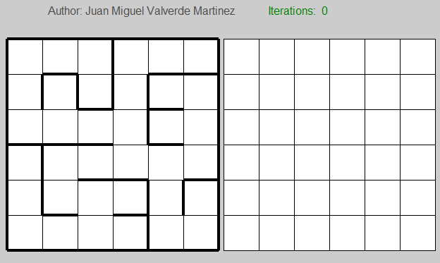
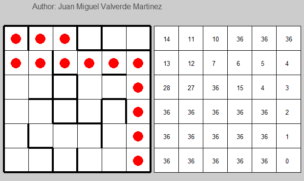
The first grid clearly represents the maze, whereas the second one indicates the current V(s) value of each state. Back to the representation of the maze, here you can see the matrix I used for store whether or not you face a wall (and therefore you can go further).
In this case, I followed the Matlab way to draw annotations, and the first row of the matrix represents the last row in the maze. As you can see in the last horizontal row of the maze, in the first, third, fifth and sixth, you don’t have any wall at all (represented as a 0 in the matrix), and so on.
The beauty of this algorithm lies in that using this two matrices and given the state or position you are, you can easily determine which states you can reach. I simply made 4 cases for up, down, left and right movements, taking special care about the borders.
The Monte Carlo algorithm
Based on this algorithm, I slightly modified it to adapt the requirements of this particular problem. In the first-visit algorithm, you have to find the first time that each state appears given an episode (for many episodes). After you find it, you have to take that particular reward or return and average it with the rest of them. In this case, I think it is not necessary to average anything, since I just want to get the minimum value. My V(s) matrix starts having a 36 value in each cell (because 36 is big enough and it’s the total amount of states).
Generating an episode
I used a ɛ-greedy version, meaning that there is a small probability ɛ that I don’t choose the best option but a random action instead. Generating an episode is quite easy: I start always in the state 1 (or 1,1 position). In the loop which lasts until I reach the state 36 (6,6 position) I call a function “pickActions” which gives me a Nx2 matrix where N is the amount of options and the columns are: state V(s). This matrix is sort by V(s) so that the best options (the minimum V(s) value) are in the top. After this, I take a random number and check it whether ɛ is bigger than that number. If ɛ is lower than the random number (most of the cases since it usually takes a value of .1 or so) I take a random option among the best actions I can do. If it’s not, I randomly pick up another action.
Time to learn
When the episode is generated, it’s time to learn. I perform a loop over the 36 different states in order to find the last of the them (or the first if I flip the vector). After I get its position, I subtract it from the length of the vector. Why I do this? It’s easy to see:
The last element will be 36, so if I subtract its index to the total length, the value will be 0, which is the highest reward. The previous element, will have a reward of 1, which is the second best reward, and so on. Then, I just need to choose the minimum value: the current value of this state or the new value I just calculated it.
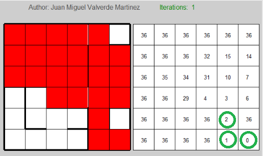
After that, I only have to update the V(s) matrix and depict it. Interestingly, I can have the best solution after the 3rd episode (in most of the cases).
One last thing that I have to say is that representing and designing simulations in Matlab gives you the great advantage of using Matlab (quite obvious) but as a disadvantage, Matlab annotations are really really slow. In the next simulation it takes terribly long just because of the graphical representation, in spite of the fact that I split the code into two parts: the first graphical drawing of the mazes, and the rest, to make it a bit faster. When I tried the algorithm without graphical representation, it takes less than 2 seconds to give you the answer.
My first idea was that you can actually see step by step the decisions of the algorithm, but it cannot be easily (and efficiently) done in Matlab, but at least you can see episode by episode.
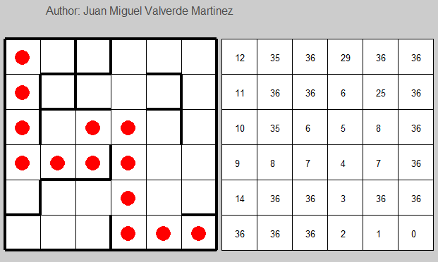
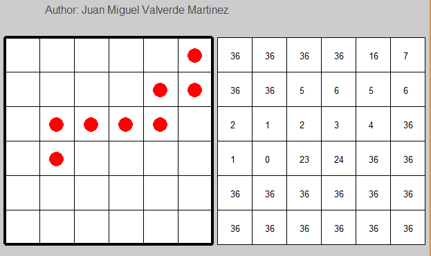
4 Random generated examples solved in 5 or less iterations. The last one is a simple path finder with no walls.

The code is provided in the Source code section.
References
1. R. S. Sutton and A. G. Barto. 2005. “Monte Carlo Methods”, Reinforcement Learning: An Introduction.