This post is the second and last part of a double entry about how SVMs work (theoretical, in practice, and implemented). You can check the first part, SVM – Support Vector Machine explained with examples.
Index
Since the algorithm uses Lagrange to optimize a function subject to certain constrains, we need a computer-oriented algorithm to implement SVMs. This algorithm called Sequential Minimal Optimization (SMO from now on) was developed by John Platt in 1998. Since it is based on Quadratic Programming (QP from now on) I decided to learn and write about it. I think it is not strictly necessary to read it, but if you want to fully understand SMO, it is recommended to understand QP, which is very easy given the example I will briefly describe.
QP is a special type of mathematical optimization problem. It describes the problem of optimizing (min or max) a quadratic function of several variables subject to linear constraints on these variables. Convex functions are used for optimization since they only have one optima which is the global optima.
Optimality conditions:
[latex]\Delta f(x^*) = 0 \quad \text{(gradient is zero, derivative)} \\
\Delta^2 f(x^*) \geq 0 \quad \text{(positive semi definite)}[/latex]
If it is a positive definite, we have a unique global minimizer. If it is a positive indefinite (or negative), then we do not have a unique minimizer.
Example
Minimize [latex]x_1^2+x_2^2-8x_1-6x_2[/latex]
[latex]\text{subject to } \quad -x_1 \leq 0 \\
\text{ } \quad \quad \quad \quad \quad -x_2 \leq 0 \\
\text{ } \quad \quad \quad \quad \quad x_1 + x_2 \leq 5
[/latex]
Initial point (where we start iterating) [latex]x_{(0)} = \begin{bmatrix}
0 \\
0
\end{bmatrix}[/latex]
Initial active set [latex]s^{(0)} = \left\{ 1,2 \right\}[/latex] (we will only take into account these constraints).
Since a quadratic function looks like: [latex]f(x) = \frac{1}{2}x^T Px + q^T x[/latex]
We have to configure the variables as:
[latex]
P = \begin{bmatrix}
2 & 0 \\
0 & 2
\end{bmatrix}
q = \begin{bmatrix}
-8 \\
-6
\end{bmatrix}
\text{(minimize)} \\
A_0 = \begin{bmatrix}
-1 & 0 \\
0 & -1 \\
1 & 1
\end{bmatrix}
b_0 = \begin{bmatrix}
0 \\
0 \\
5
\end{bmatrix}
\text{(constraints)}
[/latex]

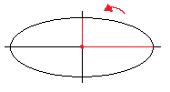
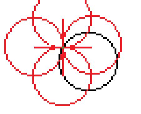
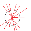
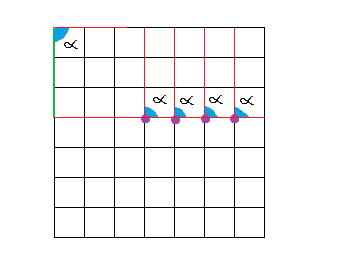
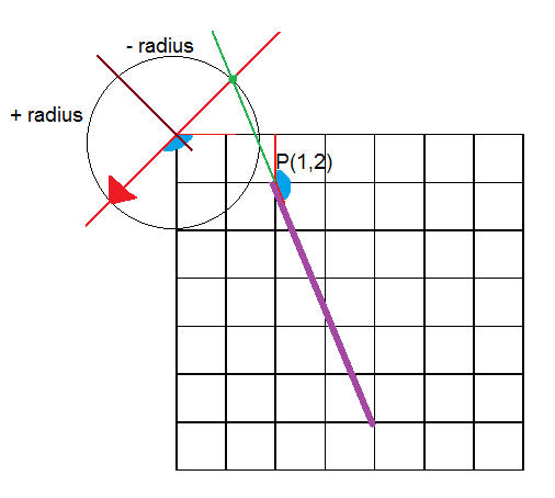
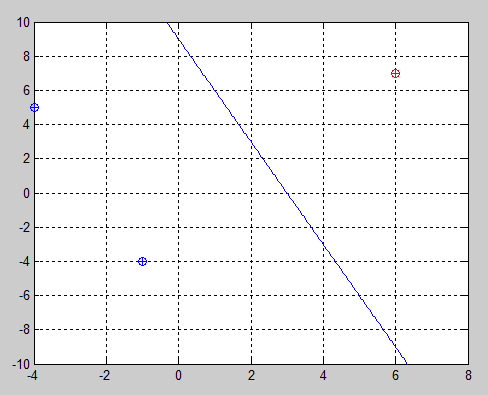
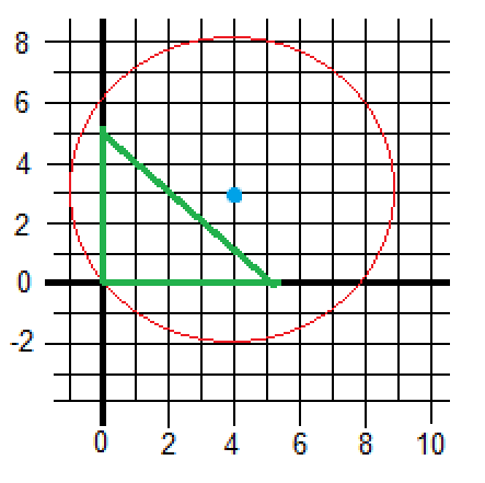
This picture represents how the problem looks like. The function we want to minimize is the red circumference whereas the green lines represent the constraints. Finally, the blue mark shows where the center and the minima are located.
Iteration 1
[latex]s^{(0)} = \left\{ 1,2 \right\} \quad \quad x_{(0)} = \begin{bmatrix}
0 \\
0
\end{bmatrix}[/latex]
Solve EQP defined by [latex]s^{(0)}[/latex], so we have to deal with the first two constraints. KKT method is used since it calculates the Lagrangian multipliers.
[latex]KKT = \begin{bmatrix}
P & A^T \\
A & 0
\end{bmatrix}
\quad \quad
\begin{bmatrix}
P & A^T \\
A & 0
\end{bmatrix}
\begin{bmatrix}
x^* \\
v^*
\end{bmatrix}
=
\begin{bmatrix}
-q \\
b
\end{bmatrix} \\
\begin{bmatrix}
2 & 0 & -1 & 0 \\
0 & 2 & 0 & -1 \\
-1 & 0 & 0 & 0 \\
0 & -1 & 0 & 0
\end{bmatrix}
\cdot
\begin{bmatrix}
x_1^* \\
x_2^* \\
v_1^* \\
v_2^*
\end{bmatrix}
=
\begin{bmatrix}
0 \\
0 \\
-8 \\
-6
\end{bmatrix}
\to
\text{Solution: }
x_{EQP}^* = \begin{bmatrix}
0 \\
0
\end{bmatrix}
v_{EQP}^* = \begin{bmatrix}
-8 \\
-6
\end{bmatrix}
[/latex]
[latex]x_{EQP}^*[/latex] indicates the next point the algorithm will iterate.
Now it is necessary to check whether this solution is feasible: [latex]A_0 \cdot x_{EQP}^* \leq b_0[/latex]
[latex]
\begin{bmatrix}
-1 & 0\\
0 & -1 \\
1 & 1
\end{bmatrix}
\cdot
\begin{bmatrix}
0\\
0
\end{bmatrix}
\leq
\begin{bmatrix}
0\\
0 \\
5
\end{bmatrix}
\to
\begin{bmatrix}
1\\
1 \\
1
\end{bmatrix}
[/latex]
It is clear that this point was going to be feasible because the point (0,0) is where we started.
Now, we remove a constraint with negative [latex]v_{EQP}^*[/latex] and move to the next value [latex]x_{EQP}^*[/latex].
[latex]S^{(1)} = S^{(0)} – \left\{\ 1 \right\} = \left\{ 2 \right\} \quad \text{constraint 1 is removed} \\
X^{(1)} = x_{EQP}^* = \begin{bmatrix}
0\\
0
\end{bmatrix}[/latex]
Graphically, we started on (0,0) and we have to move to the same point (0,0). The removal of the constraint indicates to which axis and direction we are going to move: up or right. Since we took the first constraint out, we will move to the right. Now we need to minimize constrained to the second constraint.
Iteration 2
[latex]s^{(1)} = \left\{ 2 \right\} \quad \quad x_{(1)} = \begin{bmatrix}
0 \\
0
\end{bmatrix}[/latex]
Solve EQP defined with [latex]A = \begin{bmatrix}
0 & -1
\end{bmatrix} \quad b = [0][/latex]
[latex]
K = \begin{bmatrix}
2 & 0 & 0 \\
0 & 2 & -1 \\
0 & -1 & 0
\end{bmatrix}
\cdot
\begin{bmatrix}
x_1^* \\
x_2^* \\
v_1^*
\end{bmatrix}
=
\begin{bmatrix}
8 \\
6 \\
0
\end{bmatrix}
\to
\text{Solution: }
x_{EQP}^* = \begin{bmatrix}
4 \\
0
\end{bmatrix}
\quad
v_{EQP}^* = \begin{bmatrix}
-6
\end{bmatrix}
[/latex]
Check whether this is feasible: [latex]A_0 \cdot x_{EQP}^* \leq b_0[/latex] ?
[latex]
\begin{bmatrix}
-1 & 0\\
0 & -1 \\
1 & 1
\end{bmatrix}
\cdot
\begin{bmatrix}
4 \\
0
\end{bmatrix}
=
\begin{bmatrix}
-4 \\
0 \\
4
\end{bmatrix}
\leq
\begin{bmatrix}
0\\
0 \\
5
\end{bmatrix}
\to
\begin{bmatrix}
1\\
1 \\
1
\end{bmatrix}
\quad
\text{It is feasible}
[/latex]
[latex]S^{(2)} = S^{(1)} – \left\{\ 2 \right\} = \varnothing \quad \quad \text{constraint 2 is removed} \\
X^{(2)} = \begin{bmatrix}
4\\
0
\end{bmatrix}[/latex]
Iteration 3
[latex]s^{(2)} = \varnothing \quad \quad x_{(2)} = \begin{bmatrix}
4 \\
0
\end{bmatrix}[/latex]
Solve EQP defined with [latex]A = [] \quad b = [][/latex]
[latex]
K = \begin{bmatrix}
2 & 0 \\
0 & 2
\end{bmatrix}
\cdot
\begin{bmatrix}
x_1^* \\
x_2^*
\end{bmatrix}
=
\begin{bmatrix}
8 \\
6
\end{bmatrix}
\to
\text{Solution: }
x_{EQP}^* = \begin{bmatrix}
4 \\
3
\end{bmatrix}
[/latex]
Check whether this is feasible: [latex]A_0 * x_{EQP}^* \leq b_0 = \begin{bmatrix}
1\\
1 \\
0
\end{bmatrix}[/latex]
It is not feasible. 3rd constrained is violated (that is why the third element is 0). As it is not feasible, we have to maximize [latex]\text{t} \quad \text{s.t.} \quad x^{(2)}+t(x_{EQP}^* – x^{(2)}) \in \text{Feasible}[/latex]
[latex]A_0(\begin{bmatrix}
4\\
0
\end{bmatrix}+t(\begin{bmatrix}
4\\
3
\end{bmatrix}-\begin{bmatrix}
4\\
0
\end{bmatrix})) \leq b_0 \\
\vspace{2em}
[/latex]
[latex]
\begin{bmatrix}
-1 & 0 \\
0 & -1 \\
1 & 1
\end{bmatrix}
\cdot
\begin{bmatrix}
4 \\
3t
\end{bmatrix}
\leq
\begin{bmatrix}
0 \\
0 \\
5
\end{bmatrix}
\\
-4 \leq 0 \quad \text{This is correct} \\
-3t \leq 0 \quad \text{This is correct, since} \quad 0 \leq t \leq 1 \\
4 -3t \leq 5 \quad \to \quad t = \frac{1}{3} \quad \text{(the largest)}
[/latex]
So, [latex]x^{(3)} = x^{(2)} + \frac{1}{3} (x_{EQP}^* – x^{(2)}) = \begin{bmatrix}
4 \\
1
\end{bmatrix}[/latex]
Finally we add the constraint that was violated.
[latex]S^{(2)} = S^{(1)} + \left\{\ 3 \right\} = \left\{\ 3 \right\}[/latex]
Iteration 4
[latex]s^{(3)} = \left\{ 3 \right\} \quad \quad x_{(3)} = \begin{bmatrix}
4 \\
1
\end{bmatrix}[/latex]
Solve EQP defined with [latex]A = \begin{bmatrix}
1 & 1
\end{bmatrix} \quad b = [5][/latex]
[latex]
K = \begin{bmatrix}
2 & 0 & 1 \\
0 & 2 & 1 \\
1 & 1 & 0
\end{bmatrix}
\cdot
\begin{bmatrix}
x_1^* \\
x_2^* \\
v_1^*
\end{bmatrix}
=
\begin{bmatrix}
8 \\
6 \\
5
\end{bmatrix}
\to
\text{Solution: } x_{EQP}^* = \begin{bmatrix}
3 \\
2
\end{bmatrix}
\quad
v_{EQP}^* = \begin{bmatrix}
3
\end{bmatrix}
[/latex]
Check whether this is feasible: [latex]A_0 \cdot x_{EQP}^* \leq b_0 = \begin{bmatrix}
1\\
1 \\
1
\end{bmatrix}
\quad \text{It is feasible}
[/latex]
[latex]v^* \geq 0 \quad \to \quad \text{We found the optimal}[/latex]
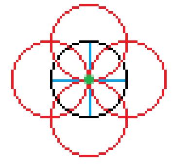
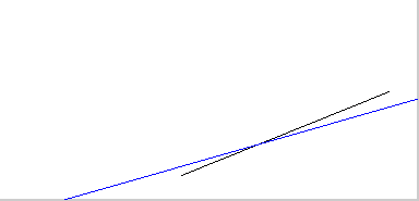
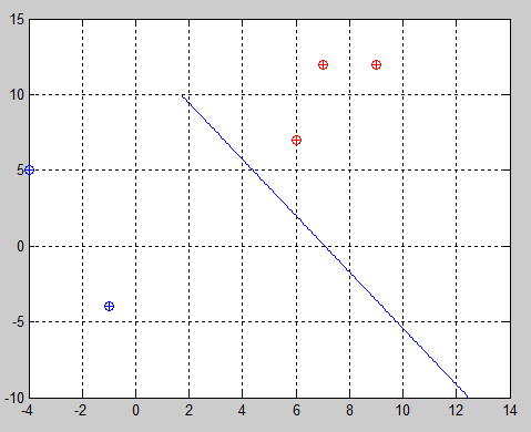
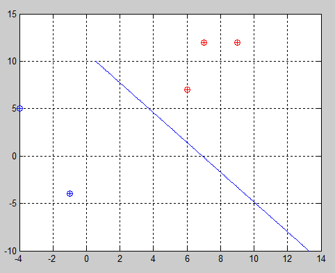
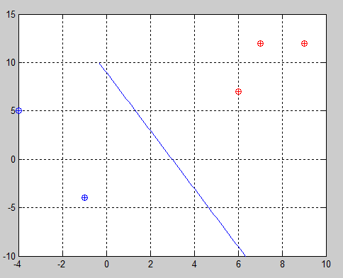
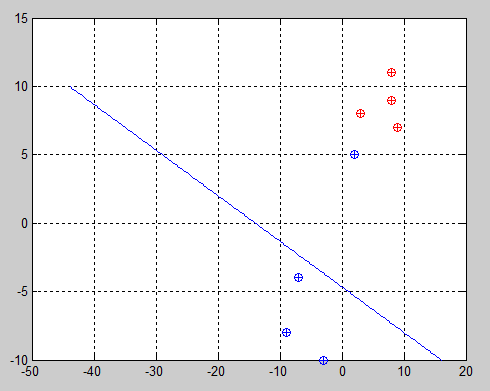
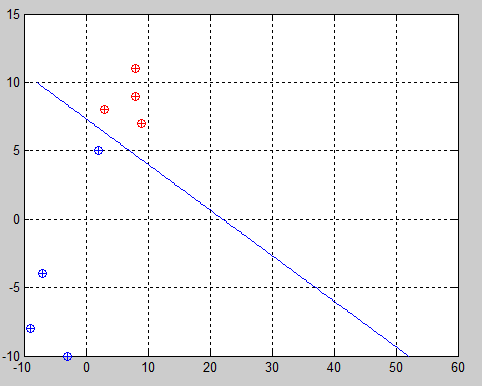
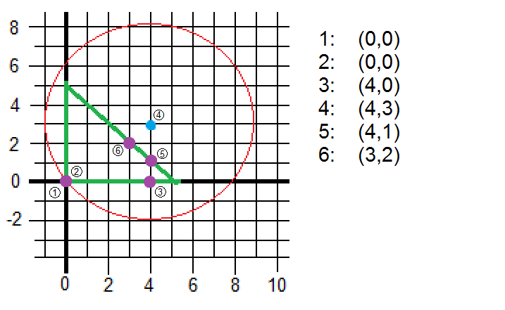
Iterations and steps are drawn on the plane below. It is graphically easy to see that the 4th step was illegal since it was out of the boundaries.
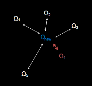
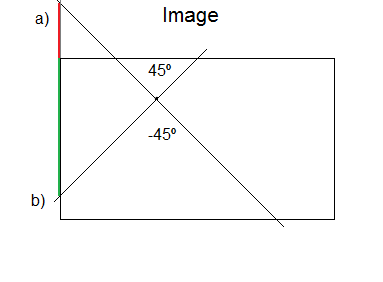
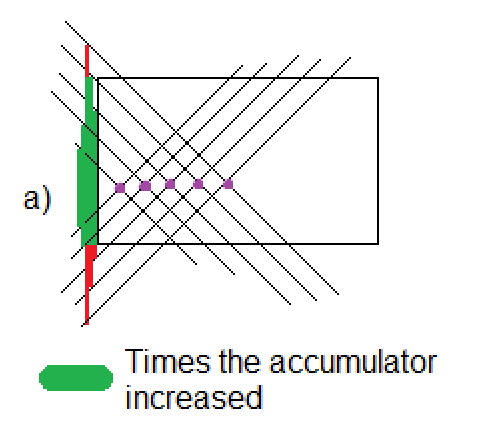
SMO is an algorithm for solving the QP problem that arises during the SVM training. The algorithm works as follows: it finds a Lagrange multiplier [latex]\alpha_i[/latex] that violates the KKT conditions for the optimization problem. It picks a second multiplier [latex]\alpha_j[/latex] and it optimizes the pair [latex](\alpha_i,\alpha_j)[/latex], and repeat this until convergence. The algorithm iterates over all [latex](\alpha_i,\alpha_j)[/latex] pairs twice to make it easier to understand, but it can be improved when choosing [latex]\alpha_i[/latex] and [latex]\alpha_j[/latex].
Because [latex]\sum_{i=0} y_i \alpha_i = 0[/latex] we have that for a pair of [latex](\alpha_1,\alpha_2): y_1 \alpha_1 + y_2 \alpha_2 = y_1 \alpha_1^{old + y_2 \alpha_2^{old}}[/latex]. This confines optimization to be as the following lines show:
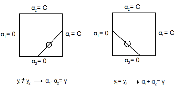
Let [latex]s = y_1 y_2[/latex] (assuming that [latex]y_i \in \left\{ -1,1 \right\}[/latex])
[latex]y_1 \alpha_1 + y_2 \alpha_2 = \text{constant} = \alpha_1 + s \alpha_2 \quad \to \quad \alpha_1 = \gamma – s \alpha_2 \\
\gamma \equiv \alpha_1 + s \alpha_2 = \alpha_1^{old} + s \alpha_2^{old} = \text{constant}[/latex]
We want to optimize:
[latex]L = \frac{1}{2} \| w \| ^2 – \sum \alpha_i [y_i (\overrightarrow{w} \cdot \overrightarrow{x_i} +b)-1] = \sum \alpha_i – \frac{1}{2} \sum_i \sum_j \alpha_i \alpha_j y_i y_j \overrightarrow{x_i} \cdot \overrightarrow{x_j}[/latex]
If we pull out [latex]\alpha_1[/latex] and [latex]\alpha_2[/latex] we have:
[latex]L = \alpha_1 + \alpha_2 + \text{const.} – \frac{1}{2}(y_1 y_1 \overrightarrow{x_1}^T \overrightarrow{x_1} \alpha_1^2 + y_2 y_2 \overrightarrow{x_2}^T \overrightarrow{x_2} \alpha_2^2 + 2 y_1 y_2 \overrightarrow{x_1}^T \overrightarrow{x_2} \alpha_1 \alpha_2 + 2 (\sum_{i=3}^N \alpha_i y_i \overrightarrow{x_i})(y_1 \overrightarrow{x_1} \alpha_1 + y_2 \overrightarrow{x_2} \alpha_2) + \text{const.} )[/latex]
Let [latex]K_{11} = \overrightarrow{x_1}^T\overrightarrow{x_1}, K_{22} = \overrightarrow{x_2}^T\overrightarrow{x_2}, K_{12} = \overrightarrow{x_1}^T\overrightarrow{x_2} \quad \text{(kernel)}[/latex] and:
[latex]v_j = \sum_{i=3}^N \alpha_i y_i \overrightarrow{x_i}^T\overrightarrow{x_j} = \overrightarrow{x_j}^T\overrightarrow{w}^{old} – \alpha_1^{old} y_1 \overrightarrow{x_1}^T \overrightarrow{x_j} – \alpha_2^{old} y_2 \overrightarrow{x_2}^T \overrightarrow{x_j}[/latex]
It represents the original formula [latex]\overrightarrow{x_j}^T\overrightarrow{w}^{old}[/latex] without the first and second [latex]\alpha[/latex]
[latex]… = \overrightarrow{x_j}^T\overrightarrow{w}^{old} -b^{old} +b^{old} – \alpha_1^{old} y_1 \overrightarrow{x_1}^T \overrightarrow{x_j} – \alpha_2^{old} y_2 \overrightarrow{x_2}^T \overrightarrow{x_j} [/latex]
Let [latex]u_j^{old} = \overrightarrow{x_j}^T\overrightarrow{w}^{old} -b^{old}[/latex]. This means that [latex]u_j^{old}[/latex] is the output of [latex]\overrightarrow{x_j}[/latex] under old parameters.
[latex]u_j^{old} + b^{old} – \alpha_1^{old} y_1 \overrightarrow{x_1}^T \overrightarrow{x_j} – \alpha_2^{old} y_2 \overrightarrow{x_2}^T \overrightarrow{x_j}[/latex]
Now we substitute in our original formula with [latex]\alpha_1[/latex] and [latex]\alpha_2[/latex] pulled out using new variables: [latex]s,\gamma,K_{11},K_{22},K_{12},v_j[/latex].
[latex]L = \alpha_1 + \alpha_2 – \frac{1}{2}(K_{11} \alpha_1^2 + K_{22} \alpha_2 + 2 s K_{12} \alpha_1 \alpha_2 + 2 y_1 v_1 \alpha_1 + 2 y_2 v_2 \alpha_2) + \text{const.}[/latex]
Note that here we assume that [latex]y_i \in \left\{ -1,1 \right\} \quad \text{since} \quad y_1^2 = y_2^2 = 1[/latex]
Now we substitute using [latex]\alpha_1 = \gamma – s \alpha_2[/latex]
[latex]L = \gamma – s \alpha_2 + \alpha_2 – \frac{1}{2} (K_{11}(\gamma – s \alpha_2)^2 + K_{22} \alpha_2^2 + 2 s K_{12}(\gamma – s \alpha_2) \alpha_2 + 2 y_1 v_1 (\gamma – s \alpha_2) +2 y_2 v_2 \alpha_2 ) + \text{const.}[/latex]
The first [latex]\gamma[/latex] is a constant so it will be added to the [latex]\text{const.}[/latex] value.
[latex] L = (1 -s) \alpha_2 – \frac{1}{2} K_{11} (\gamma – s \alpha_2)^2 – \frac{1}{2} K_{22} \alpha_2^2 – s K_{12} (\gamma -s \alpha_2) \alpha_2 – y_1 v_1 (\gamma – s \alpha_2) – y_2 v_2 \alpha_2 + \text{const.} \\
= (1 -s) \alpha_2 – \frac{1}{2} K_{11} \gamma^2 + s K_{11} \gamma \alpha_2 – \frac{1}{2} K_{11} s^2 \alpha_2^2 – \frac{1}{2} K_{22} \alpha_2^2 – s K_{12} \gamma \alpha_2 + s^2 K_{12} \alpha_2^2 – y_v v_1 \gamma + s y_1 v_1 \alpha_2 – y_2 v_2 \alpha_2 + \text{const.}[/latex]
Constant terms are grouped and [latex]y_2 = \frac{s}{y_1}[/latex] is applied:
[latex](1 -s) \alpha_2 + s K_{11} \gamma \alpha_2 – \frac{1}{2} K_{11} \alpha_2^2 – \frac{1}{2} K_{22} \alpha_2^2 – s K_{12} \gamma \alpha_2 + K_{12} \alpha_2^2 + y_2 v_1 \alpha_2 – y_2 v_2 \alpha_2 + \text{const.} \\
= (- \frac{1}{2} K_{11} – \frac{1}{2} K_{22} + K_{12}) \alpha_2^2 + (1-s+s K_{11} \gamma – s K_{12} + y_2 v_1 – y_2 v_2) \alpha_2 + \text{const.} \\
= \frac{1}{2}(2 K_{12} – K_{11} – K_{22}) \alpha_2^2 + (1 -s +s K_{11} \gamma – s K_{12} \gamma + y_2 v_1 – y_2 v_2) \alpha_2 + \text{const.}
[/latex]
Let [latex]\eta \equiv 2 K_{12} – K_{11} – K_{12}[/latex]. Now, the formula is reduced to [latex]\frac{1}{2} \eta \alpha_2^2 + (\dots)\alpha_2 + \text{const.}[/latex]. Let us focus on the second part (the coefficient “[latex]\dots[/latex]”). Remember that [latex]\gamma = \alpha_1^{old} + s \alpha_2^{old}[/latex]
[latex]1 -s +s K_{11} \gamma – s K_{12} \gamma + y_2 v_1 – y_2 v_2 \\
= 1 – s + s K_{11}(\alpha_1^{old}+s \alpha_2^{old}) – s K_{12} (\alpha_1^{old}+s \alpha_2^{old}) \\
\hspace{6em} \text{ } + y_2 (u_1^{old}+b^{old} – \alpha_1^{old} y_1 K_{11} – \alpha_2^{old} y_2 K_{12}) \\
\hspace{6em} \text{ } – y_2 (u_2^{old}+b^{old} – \alpha_1^{old} y_1 K_{12} – \alpha_2^{old} y_2 K_{22}) \\
= 1 – s + s K_{11}\alpha_1^{old}+ K_{11} \alpha_2^{old} – s K_{12} \alpha_1^{old} – K_{12} \alpha_2^{old} \\
\hspace{6em} \text{ } + y_2 u_1^{old} + y_2 b^{old} – s \alpha_1^{old} K_{11} – \alpha_2^{old} K_{12} \\
\hspace{6em} \text{ } – y_2 u_2^{old} – y_2 b^{old} + s \alpha_1^{old} K_{12} + \alpha_2^{old} K_{22} \\
= 1 -s +(s K_{11} – s K_{12} – s K_{11} + s K_{12}) \alpha_1^{old} \\
\hspace{6em} \text{ } + (K_{11} – 2 K_{12} + K_{22}) \alpha_2^{old} + y_2 (u_1^{old} – u_2^{old})
[/latex]
Since [latex]y_2^2 = 1[/latex]: (mathematical convenience)
[latex]y_2^2 – y_1 y_2 + (K_{11} – 2 K_{12} + K_{11} + s K_{12}) \alpha_2^{old} + y_2(u_1^{old} – u_2^{old}) \\
= y_2 (y_2 – y_1 + u_1^{old} – u_2^{old}) – \eta \alpha_2^{old} \\
= y_2 ((u_1^{old} – y_1) – (u_2^{old} – y_2)) – \eta \alpha_2^{old} \\
= y_2 (E_1^{old} – E_2^{old}) – \eta \alpha_2^{old}
[/latex]
Therefore, the objective function is:
[latex]\frac{1}{2} \eta \alpha_2^2 + (y_2 (E_1^{old} – E_2^{old}) – \eta \alpha_2^{old}) + \text{const.}[/latex]
First derivative: [latex]\frac{\partial L}{\partial \alpha_2} = \eta \alpha_2 + (y_2 (E_1^{old} – E_2^{old}) – \eta \alpha_2^{old})[/latex]
Second derivative: [latex]\frac{\partial^2 L}{\partial \alpha_2} = \eta[/latex]
Note that [latex]\eta = 2 K_{12} – K_{11} – K_{22} \leq 0[/latex]. Proof: Let [latex]K_{11} = \overrightarrow{x_1}^T \overrightarrow{x_1}, K_{12} = \overrightarrow{x_1}^T \overrightarrow{x_2}, K_{22} = \overrightarrow{x_2}^T \overrightarrow{x_2}[/latex]. Then [latex]\eta = – (\overrightarrow{x_2} – \overrightarrow{x_1})^T (\overrightarrow{x_2} – \overrightarrow{x_1}) = -\|\overrightarrow{x_2} – \overrightarrow{x_1} \| \leq 0[/latex]
This is important to understand because when we want to use other kernels this has to be true.
[latex]\text{Let} \quad \frac{\partial L}{\partial \alpha_2} = 0, \text{then we have that} \\
\text{ } \quad \alpha_2^{new} = \frac{- y_2 (E_1^{old} – E_2^{old}) – \eta \alpha_2^{old}}{\eta}[/latex]
Therefore, this is the formula to get a maximum:
[latex]\alpha_2^{new} = \alpha_2^{old} + \frac{y_2 (E_2^{old} – E_1^{old})}{\eta}[/latex]
While performing the algorithm, after calculating [latex]\alpha_j[/latex] (or [latex]\alpha_2[/latex]) it is necessary to clip its value since it is constrained by [latex]0 \leq \alpha_i \leq C[/latex]. This constraint comes from the KKT algorithm.
So we have that: [latex]\text{ } \quad s=y_1 y_2 \quad \gamma = \alpha_1^{old} + s \alpha_2^{old}[/latex]
If [latex]s=1[/latex], then [latex]\alpha_1 + \alpha_2 = \gamma[/latex]
If [latex]\gamma > C[/latex], then [latex]\text{max} \quad \alpha_2 = C, \text{min} \quad \alpha_2 = \gamma – C[/latex]
If [latex]\gamma < C[/latex], then [latex]\text{min} \quad \alpha_2 = 0, \text{max} \quad \alpha_2 = \gamma[/latex]
If [latex]s=-1[/latex], then [latex]\alpha_1 – \alpha_2 = \gamma[/latex]
If [latex]\gamma > 0[/latex], then [latex]\text{min} \quad \alpha_2 = 0, \text{max} \quad \alpha_2 = C – \gamma[/latex]
If [latex]\gamma < 0[/latex], then [latex]\text{min} \quad \alpha_2 = - \gamma, \text{max} \quad \alpha_2 = C[/latex]
In other words: (L = lower bound, H = higher bound)
[latex]
\text{If} \quad y^{(i)} \neq y^{(j)}, L = max(0,\alpha_j – \alpha_i), H = min(C, C+ \alpha_j – \alpha_i) \\
\text{If} \quad y^{(i)} = y^{(j)}, L = max(0,\alpha_i + \alpha_j – C), H = min(C, \alpha_i + \alpha_j)
[/latex]
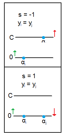
Why do we need to clip our [latex]\alpha_2[/latex] value?
We can understand it using a very simple example.
Remember that if [latex]y_1 = y_2[/latex], then [latex]s = 1 \quad \text{and} \quad \gamma = \alpha_1^{old} + s \alpha_2^{old}[/latex] remains always constant. If [latex]y_2 \neq y_2[/latex], then [latex]\alpha_1 = \alpha_2[/latex] so they can change as much as they want if they remain equal. In the first case, the numbers are balanced, so if [latex]\alpha_1 = 0.2 \quad \text{and} \quad \alpha_2 = 0.5[/latex], as they sum 0.7, they can change maintaining that constraint true, so they may end up being [latex]\alpha_1 = 0.4, \alpha_2 = 0.3[/latex].
If [latex]\alpha_1 = 0.3, \alpha_2 = 0.4, C = 1[/latex]:
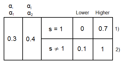
1) As explained before, and taking into account that [latex]\Delta \alpha_1 = -s \Delta \alpha_2[/latex], [latex]\alpha_2[/latex] can only increase 0.3 because [latex]\alpha_1[/latex] can only decrease 0.3 keeping this true: [latex]0 \leq \alpha_1 \leq C[/latex]. Likewise, [latex]\alpha_2[/latex] can only decrease 0.4 because [latex]\alpha_1[/latex] can only increase that amount.
2) If they are different, [latex]\alpha_2[/latex] can grow up to 1 because similarly, [latex]\alpha_1[/latex] will grow up to 1 (which is the value of C and hence, the upper boundary). [latex]\alpha_1[/latex] can only decrease till 0.1 because if it decreases till 0, [latex]\alpha_1[/latex] would be -0.1 and the constraint would be violated.
Remember that the reason why [latex]\alpha_1[/latex] has to be [latex]0 \leq \alpha_1 \leq C[/latex] is because of the KKT algorithm.
| [latex]\alpha_i[/latex] |
[latex]\alpha_j[/latex] |
s |
L |
H |
| 0 |
1 |
-1 |
1 |
1 |
|
|
If [latex]L == M[/latex], it means that we cannot balance or proportionally increase/decrease at all between [latex]\alpha_i[/latex] and [latex]\alpha_j[/latex]. In this case, we skip this [latex]\alpha_i – \alpha_j[/latex] combination and try a new one.
|
After updating [latex]\alpha_i[/latex] and [latex]\alpha_j[/latex] we still need to update b.
[latex]\sum (x,y) = \sum_{i=1}^N \alpha_i y_i \overrightarrow{x_i}^T\overrightarrow{x} -b -y[/latex] (the increment of a variable is given by the increment of all variables which are part of it).
[latex]\Delta \sum (x,y) = \Delta \alpha_1 y_1 \overrightarrow{x_1}^T\overrightarrow{x} + \Delta \alpha_2 y_2 \overrightarrow{x_2}^T\overrightarrow{x} – \Delta b[/latex]
The change in the threshold can be computed by forcing [latex]E_1^{new} = 0 \text{ if } 0 < \alpha_1^{new} < C \text{(or } E_2^{new} = 0 \text{ if } 0 < \alpha_2^{new} < C \text{)}[/latex]
[latex]E (x,y)^{new} = 0 \\
E(x,y)^{old} + \Delta E (x,y) = E (x,y)^{old} + \Delta \alpha_1 y_1 \overrightarrow{x_1}^T \overrightarrow{x} + \Delta \alpha_2 y_2 \overrightarrow{x_2}^T \overrightarrow{x} - \Delta b[/latex]
So we have:
[latex]\Delta b = E(x,y)^{old} + \Delta \alpha_1 y_1 \overrightarrow{x_1}^T \overrightarrow{x} + \Delta \alpha_2 y_2 \overrightarrow{x_2}^T \overrightarrow{x}[/latex]
The code I provide in the Source code section was developed by me, but I followed the algorithm shown in [1]. I will copy the algorithm here since it made my life really easier and avoided me many headaches for sure. All the credit definitely goes to the writer.
Algorithm: Simplified SMO
Note: if you check [1] you will see that this algorithm differs from the original one written on that paper. The reason is because the original one had mistakes that I wanted to fix and improve. I talk about that in this post.
Input:
C: regularization parameter
tol: numerical tolerance
max_passes: max # of times to iterate over [latex]\alpha[/latex]’s without changing
[latex](x^{(1)},y^{(1)}),…,(x^{(m)},y^{(m)})[/latex]: training data
Output:
[latex]\alpha \in \mathbb{R}^m[/latex]: Lagrange for multipliers for solution
[latex]b \in \mathbb{R}[/latex]: threshold for solution
Algorithm:
Initialize [latex]\alpha_i = 0, \forall i, b = 0[/latex]
Initialize [latex]\text{counter} = 0[/latex]
[latex]\text{while} ((\exists x \in \alpha | x = 0 ) \text{ } \& \& \text{ } (\text{counter} < \text{max\_iter}))[/latex]
Initialize input and [latex]alpha[/latex]
[latex]\text{for } i = 1, … numSamples[/latex]
Calculate [latex]E_i = f(x^{(i)}) – y^{(i)}[/latex] using (2)
[latex]\text{if } ((y^{(i)} E_i < -tol \quad \& \& \quad \alpha_i < C) \| (y^{(i)} E_i > tol \quad \& \& \quad \alpha_i > 0))[/latex]
[latex]\text{for } j = 1, … numSamples \quad \& \quad j \neq i[/latex]
Calculate [latex]E_j = f(x^{(j)}) – y^{(j)}[/latex] using (2)
Save old [latex]\alpha[/latex]’s: [latex]\alpha_i^{(old)} = \alpha_i, \alpha_j^{(old)} = \alpha_j[/latex]
Compute [latex]L[/latex] and [latex]H[/latex] by (10) and (11)
[latex]\text{if } (L == H)[/latex]
Continue to [latex]\text{next j}[/latex]
Compute [latex]\eta[/latex] by (14)
[latex]\text{if } (\eta \geq 0)[/latex]
Continue to [latex]\text{next j}[/latex]
Compute and clip new value for [latex]\alpha_j[/latex] using (12) and (15)
[latex]\text{if } (| \alpha_j – \alpha_j^{(old)} < 10^{-5})[/latex] (*A*)
Continue to [latex]\text{next j}[/latex]
Determine value for [latex]\alpha_i[/latex] using (16)
Compute [latex]b_1[/latex] and [latex]b_2[/latex] using (17) and (18) respectively
Compute [latex]b[/latex] by (19)
[latex]\text{end for}[/latex]
[latex]\text{end if}[/latex]
[latex]\text{end for}[/latex]
[latex]\text{counter } = \text{ counter}++[/latex]
[latex]\text{data } = \text{ useful\_data}[/latex] (*B*)
[latex]\text{end while}[/latex]
Algorithm Legend
(*A*): If the difference between the new [latex]\alpha[/latex] and [latex]\alpha^{(old)}[/latex] is negligible, it makes no sense to update the rest of variables.
(*B*): Useful data are those samples whose [latex]\alpha[/latex] had a nonzero value during the previous algorithm iteration.
(2): [latex]f(x) = \sum_{i=1}^m \alpha_i y^{(i)} \langle x^{(i)},x \rangle +b[/latex]
(10): [latex]\text{If } y^{(i)} \neq y^{(j)}, \quad L = \text{max }(0, \alpha_j – \alpha_i), H = \text{min } (C,C+ \alpha_j – \alpha_i)[/latex]
(11): [latex]\text{If } y^{(i)} = y^{(j)}, \quad L = \text{max }(0, \alpha_i + \alpha_j – C), H = \text{min } (C,C+ \alpha_i + \alpha_j)[/latex]
(12): [latex] \alpha_ := \alpha_j – \frac{y^{(j)}(E_i – E_j)}{ \eta }[/latex]
(14): [latex]\eta = 2 \langle x^{(i)},x^{(j)} \rangle – \langle x^{(i)},x^{(i)} \rangle – \langle x^{(j)},x^{(j)} \rangle[/latex]
(15): [latex]\alpha_j := \begin{cases} H \quad \text{if } \alpha_j > H \\
\alpha_j \quad \text{if } L \leq \alpha_j \leq H \\
L \quad \text{if } \alpha_j < L \end{cases}[/latex]
(16): [latex]\alpha_i := \alpha_i + y^{(i)} y^{(j)} (\alpha_j^{(old)} - \alpha_j)[/latex]
(17): [latex]b_1 = b - E_i - y^{(i)} (\alpha_i^{(old)} - \alpha_i) \langle x^{(i)},x^{(i)} \rangle - y^{(j)} (\alpha_j^{(old)} - \alpha_j) \langle x^{(i)},x^{(j)} \rangle[/latex]
(18): [latex]b_2 = b - E_j - y^{(i)} (\alpha_i^{(old)} - \alpha_i) \langle x^{(i)},x^{(j)} \rangle - y^{(j)} (\alpha_j^{(old)} - \alpha_j) \langle x^{(j)},x^{(j)} \rangle[/latex]
(19): [latex]\alpha_j := \begin{cases} b_1 \quad \quad \text{if } 0 < \alpha_i < C \\
b_2 \quad \quad \text{if } 0 < \alpha_j < C \\
(b_1 + b_2)/2 \quad \text{otherwise} \end{cases}[/latex]
Source Code Legend
(*1*): This error function arises when we try to see the difference between our output and the target: [latex]E_i = f(x_i) – y_i = \overrightarrow{w}^T \overrightarrow{x_i}[/latex] and as [latex]\overrightarrow{w} = \sum_i^N \alpha_i y_i x_i[/latex] we get that [latex]E_i = \sum_i^N \alpha_i y_i \overrightarrow{x} \cdot \overrightarrow{x_i} + b – y_i[/latex]
(*2*): This line has 4 parts: if ((a && b) || (c && d)). A and C parts control that you will not enter if the error is lower than the tolerance. And honestly, I don’t get parts B and D. Actually I tried to run this code with several problems and the result is always the same with and without those parts. I know that alpha is constrained to be within that range, but I don’t see the relationship between A and B parts, and C and D parts separately, because that double constraint (be greater than 0 and lower than C) should be always checked.
Given a 3D space we have two samples from each class. The last column indicates the class:
[latex]data = \begin{bmatrix}
0 & 0 & 3 & -1 \\
0 & 3 & 3 & -1 \\
3 & 0 & 0 & 1 \\
3 & 3 & 0 & 1
\end{bmatrix}[/latex]
Solution:
[latex]W = [0.3333 0 -0.3333] \to f(x,y,z) = x-z[/latex]
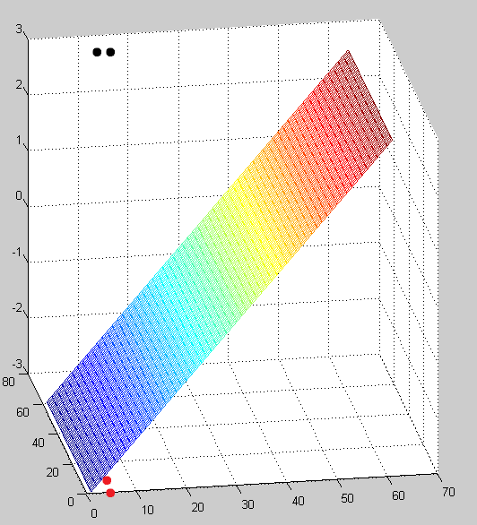
The code is provided in the Source code section.
References
1. The Simplified SMO Algorithm http://cs229.stanford.edu/materials/smo.pdf
2. Sequential Minimal Optimization for SVM http://www.cs.iastate.edu/~honavar/smo-svm.pdf
3. Inequality-constrained Quadratic Programming – Example https://www.youtube.com/watch?v=e6jDGxNZ-kk