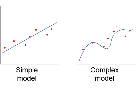
Regularization is a technique used in Machine Learning to penalize complex models. The reason why regularization is useful is because simple models generalize better and are less prone to overfitting.
Examples of regularization:
- K-means: limiting the splits to avoid redundant classes
- Random forests: limiting the tree depth, limiting new features (branches)
- Neural networks: limiting the model complexity (weights)
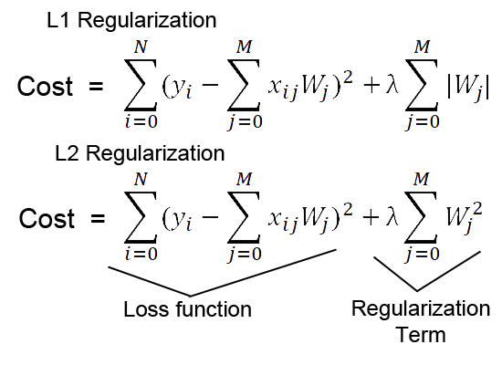
In Deep Learning there are two well-known regularization techniques: L1 and L2 regularization. Both add a penalty to the cost based on the model complexity, so instead of calculating the cost by simply using a loss function, there will be an additional element (called “regularization term”) that will be added in order to penalize complex models.
The theory
L1 regularization (LASSO regression) produces sparse matrices. Sparse matrices are zero-matrices in which some elements are ones (the sparsity refers to the ones), but in this context a sparse matrix could be several close-to-zero values and other larger values. From the data science point of view this is interesting because we can reduce the amount of features. If we find a model with neurons whose weights are close to zero it means we don’t need those neurons because the model deactivates them with zeros and we might not need a specific feature/input leading to a simpler model. For instance, if we have 50 coefficients but only 10 are non-zero, the other 40 are irrelevant to make our predictions. This is not only interesting from the efficiency point of view but also from the economic point of view: gathering data and extracting its features might be a very expensive task (in terms of time and money). Reducing this will benefit us.
Due to the absolute value, L1 regularization provides with a non-differentiable term, but despite of that, there are methods to minimize it. As we will see below, L1 regularization is also robust to outliers.
L2 regularization (Ridge regression) on the other hand leads to a balanced minimization of the weights. Since L2 uses squares, it emphasizes the errors, and it can be a problem when there are outliers in the data. Unlike L1, L2 has an analytical solution which makes it computationally efficient.
Both regularizations have a λ parameter which is directly proportional to the penalty: the larger λ the stronger penalty to find complex models and it will be more likely that the model will avoid them. Likewise, if λ is zero, regularization is deactivated.
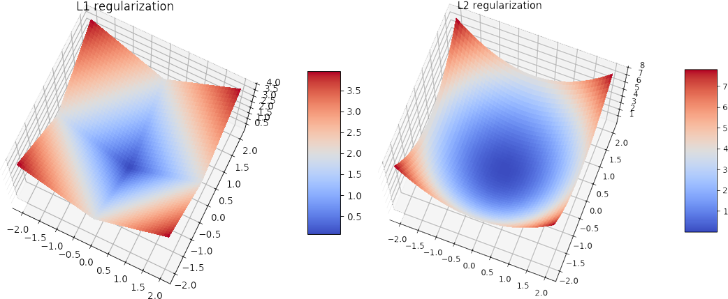
The graphs above show how the functions used in L1 and L2 regularization look like. The penalty in both cases is zero in the center of the plot, but this also implies that the weights are zero and the model will not work. The values of the weights try to be as low as possible to minimize this function, but inevitably they will leave the center and will head outside. In case of L2 regularization, going towards any direction is okay because, as we can see in the plot, the function increases equally in all directions. Thus, L2 regularization mainly focuses on keeping the weights as low as possible.
In contrast, L1 regularization’s shape is diamond-like and the weights are lower in the corners of the diamond. These corners show where one of the axis/feature is zero thus leading to sparse matrices. Note how the shapes of the functions shows their differentiability: L2 is smooth and differentiable and L1 is sharp and non-differentiable.
In few words, L2 will aim to find small weight values whereas L1 could put all the values in a single feature.
L1 and L2 regularization methods are also combined in what is called elastic net regularization.
The practice
One of my motivations to try this out was an “intuitive explanation” of L1 vs. L2 I found in quora.
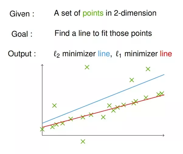
From the theoretical point of view it makes sense: L2 emphasizes errors due to the square, and it will try to minimize them all of them equally so the line will get a bit off from the main trend because a big errors influences more than small errors. On the other hand, for L1 errors have the same importance (linearly speaking) so it will minimize a lot of errors getting really close to the main train even if there are outliers.
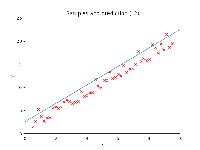
I created a small dataset of samples that describes a straight line and I later added noise and some outliers. I created a model with more neurons than needed to solve this problem in order to see whether it works and compare the weight evolution between the methods.
Model characteristics:
-Layers: 1 input, 3 hidden, 1 output
-Sizes: 1,10,10,10,1
-Batch size: 1 (noiser)
-Optimizer: SGD (lr=0.01)
-Lambda: 0.3 (for regularization)
I run the model 5 times with each regularization method and these are the results.

When the random outliers are sufficiently far none of them present good results, but overall the results obtained with L2 performance were better than those obtained with L1. Then, I had a look at the weights. Below, I show the weights and the results obtained with an additional run of the model.

|

|
|
|
As expected, L1 generates several 0-weighted neurons, so the model doesn’t use them. In other experiments, I got that most of the neurons were disconnected and only few of them had non-zero weights. On the other hand, L2 minimizes the values of the weights until most of them have a very low value.
Adjusting the network according to L1
As described before, L1 generates sparse matrices with disconnected neurons. If a neuron is disconnected, we don’t need it, leading to simpler models. I run again the script that uses L1 and I will adjust the model using less neurons according to the neurons it disconnects. Using the same samples and running the model 5 times, I got this total errors: 22.68515524, 41.64545712, 4.77383674, 24.04390211, 7.25596004.
The weights in this first run look like this:
I adjusted the neurons of the model: From [(1,10),(10,10),(10,10),(10,1)] to [(1,10),(10,10),(10,1),(1,1)] and this are the weights (note: the last big square is a single weight):
Performance on 5 runs: 7.61984439, 13.85177842, 11.95983347, 16.95491162, 25.17294774.
Implementation in Tensorflow
Despite the code is provided in the Code page as usual, implementing L1 and L2 takes very few lines: 1) Add regularization to the Weights variables (remember the regularizer returns a value based on the weights), 2) collect all the regularization losses, and 3) add to the loss function to make the cost larger.
W = tf.get_variable("W",shape=[1,10],initializer=tf.contrib.layers.xavier_initializer(),regularizer=tf.contrib.layers.l2_regularizer(lambdaReg))
...
reg_losses = tf.reduce_sum(tf.get_collection(tf.GraphKeys.REGULARIZATION_LOSSES))
cost = tf.reduce_sum(tf.abs(tf.subtract(pred, y)))+reg_losses
Conclusion
The performance of the model depends so much on other parameters, especially learning rate and epochs, and of course the number of hidden layers. Using a not-so good model, I compared L1 and L2 performance, and L2 scores were overall better than L1, although L1 has the interesting property of generating sparse matrices.
Hypothetical improvements: This post aimed to show in a very simple and graphic/animated way the effects of L1 and L2. Further research would imply trying more complex models with data that gives stable results. After tunning the parameters to get the best results, one could use cross validation to compare better the performance.
The code is provided in the Source code section.