[Reinforcement Learning] Sarsa algorithm, a practical case

Definitions

Sarsa is one of the most well-known Temporal Difference algorithms used in Reinforcement Learning. TD algorithms combine Monte Carlo ideas, in that it can learn from raw experience without a model of the environment’s dynamics, with Dynamic Programming ideas, in that their learned estimates are based on previous estimates without the need of waiting for a final outcome [1].

On-policy methods learn the value of the policy that is being used to make decisions, whereas off-policy methods learn from different policies for behavior and estimation [2].

Sarsa algorithm

On the contrary of other RL methods that are mathematically proved to converge, TD convergence depends on the learning rate α. In order to understand this, we only need to imagine the typical downhill image that comes to our minds when dealing with learning rates. If the chosen learning rate is not small enough, the error will go downhill but at some point it will go uphill. As we will see on the simulations I carried on, this may have devastating consequences as messing up the final result. Nonetheless, if the learning rate is not big enough, it won’t reach the optimal solution if we don’t iterate enough.

The algorithm is quite simple, but it’s important to understand it.

Initialize Q(s,a) arbitrarily
Repeat (for each episode):
   Initialize s
   Choose a from s using a policy derived from Q (e.g., ɛ-greedy)
   Repeat (for each step of the episode):
      Take action a, observe r, s'
      Choose a' from s' using policy derived from Q (e.g., ɛ-greedy)
      Q (s,a) ← Q(s,a) + α[r + γQ(s',a') - Q(s,a)]
      s ← s'; a ← a'
   until s is terminal

α represents the learning rate, how much does the algorithm learn each iteration.
γ represents the discounted reward, how important is the next state.
r is the reward the algorithm gets after performing action a from state s leading to state s’.
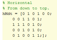
Q(s,a) stores the value of doing action a from state s. There will be 36 states and 4 different actions (1 = going up, 2 = left, 3 = down, 4 = right).

I reused the code of my previous simulation [Reinforcement Learning] First-visit Monte Carlo simulation solving a maze. To make it faster I avoided the GUI, however, it can be turned on by simply change a parameter from 0 to 1.

Noname

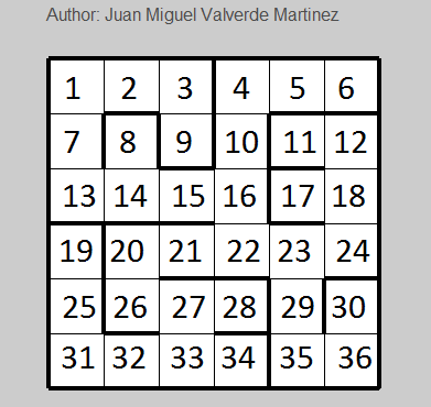
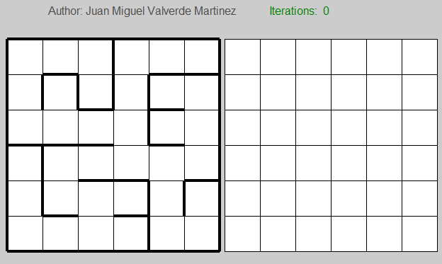
Since I am not using a graphical interface, it is worth mentioning that the numbers in the first grid represent the states, so for this maze, the optimal solution will be: 1 – 7 – 13 – 14 – 15 – 16 – 22 – 23 – 29 – 35 – 36

The algorithm has a certain number of iterations that will allow us to control how far it is going to iterate. I also established a limit of iterations for each general iteration to avoid getting stuck. In all cases I tried with γ = 1, so I consider really important the next state. In contrast, I tried with different learning rates.

Learning rate = 0.5
graph1_05

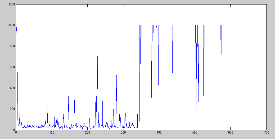
We can clearly see that it starts with many iterations, but it decreases very soon. However, after it starts increasing the iterations, it gets worse and worse. We can actually see that it surpassed the limit of 1000 iterations many times.

Learning rate = 0.3
graph1_03

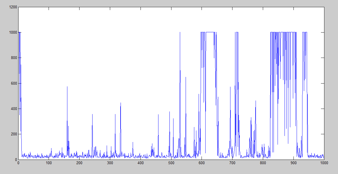
Here it is slightly better, but still terribly bad after the 150th iteration approx.

Learning rate = 0.1
graph1_01

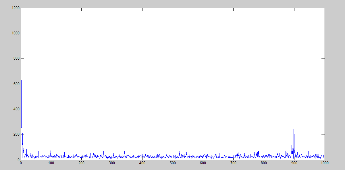
We can finally see here that the performance is way better, but still it gets worse after 875th iteration. Nonetheless, what is it being done when it starts to grow up again? In terms of the amount of iterations, we can see that peak here:

a

If we check what is going on in the state transition, we will find that it is stuck and it will be stuck until a random number lower than ɛ is generated, and therefore, try another solution.

b

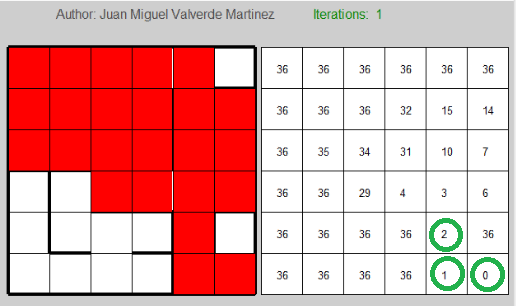
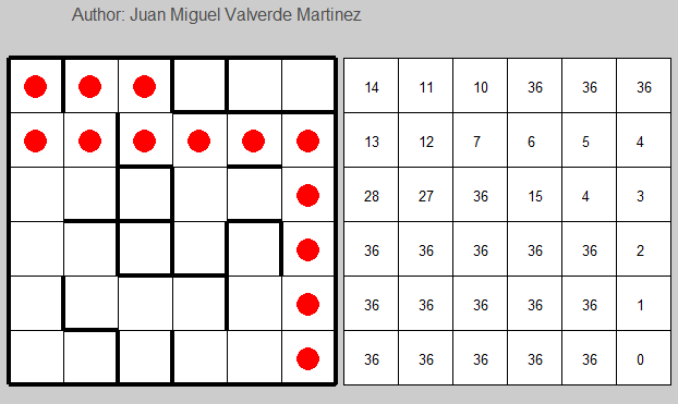
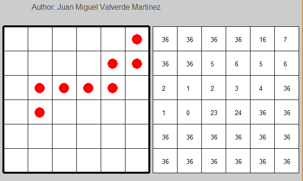
When it starts to get worse, we can stop the general iteration and check the S(a,b) values to understand what happens.

c

d

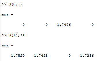
From state 8, the only option the algorithm can perform is doing the third action (going down).
From state 14, the best option is the action number 1, which means going up. Note that the correct action (left) is slightly worse: 1.752 – 1.7498 = 0.0022. Note also that that amount is smaller than the learning rate 0.01. If it learns again the correct answer, it will be fixed.

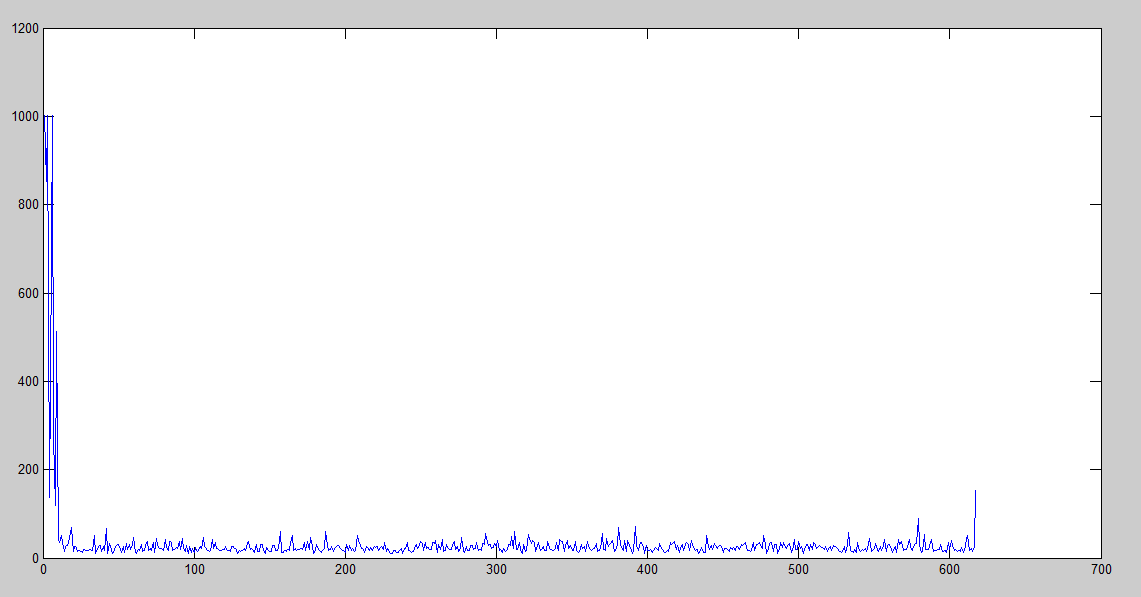
The final solution to this problem was using the following parameters:

ɛ = .3;
α = 0.1;
γ = 1;
maxCounter = 700; % Limit of general iterations

And a small trick: after the 20th general iteration it usually starts to get better, so I will add a small piece of code to tell the algorithm that if it starts to get worse after the 20th iteration, it should stop automatically before it completely messes up the solution.

if counter > 20 && counterIter > 100
   finish = 1;
end

Demonstration:

Complementary slides explaining the algorithm: Sarsa Algorithm

References

1. R. S. Sutton and A. G. Barto. 2005. “Temporal-Difference Learning”, Reinforcement Learning: An Introduction. (http://webdocs.cs.ualberta.ca/~sutton/book/ebook/node60.html)
2. http://www.cse.unsw.edu.au/~cs9417ml/RL1/tdlearning.html

[Reinforcement Learning] First-visit Monte Carlo simulation solving a maze

Recently I was reading about Monte Carlo and I decided that I had to implement one of its versions before going further to the next chapter in order to fully understand it. Personally Monte Carlo was a bit hard to understand because it’s not a simply algorithm or bunch of algorithms, but a general framework of solving problems instead. Finally, after reading the corresponding chapter [1] I went down to work and started to think and design a toy problem in Matlab.

Matlab design explanation

The most interesting thing is that I developed it very generically: you can set the start and goal state and generate a customized configuration of the walls (or randomized, or no walls at all). It only have the condition that you can only use 36 states, which I considered enough for a simulation.

I faced two problems when developing this algorithm. The first one made me lose roughly one hour since I was using relative values to draw the elements, but I finally changed to pixels because I can have an exhaustive and exact control about the size of each square. The second problem was the orientation. My mind was quite messed up thinking what should be better. The choices were: being the (1,1) element the square in the left-bottom corner (as it’s usually in the graphs that I’m used to), being the (1,1) element the square in the left-top corner (easier to deal with matrices in Matlab), and in this last case, should the first element of the matrix be the vertical distance (as it’s in the matrices in Matlab) or should I follow my intuition with the graphs? At the end, I decided to follow Matlab matrices. However, I had another small problem: when drawing in Matlab the annotation, you usually have to start from bottom to top, unlike the matrices’ indexes which start from top to bottom.

maze

The first grid clearly represents the maze, whereas the second one indicates the current V(s) value of each state. Back to the representation of the maze, here you can see the matrix I used for store whether or not you face a wall (and therefore you can go further).

hMdt

In this case, I followed the Matlab way to draw annotations, and the first row of the matrix represents the last row in the maze. As you can see in the last horizontal row of the maze, in the first, third, fifth and sixth, you don’t have any wall at all (represented as a 0 in the matrix), and so on.

The beauty of this algorithm lies in that using this two matrices and given the state or position you are, you can easily determine which states you can reach. I simply made 4 cases for up, down, left and right movements, taking special care about the borders.

The Monte Carlo algorithm

Based on this algorithm, I slightly modified it to adapt the requirements of this particular problem. In the first-visit algorithm, you have to find the first time that each state appears given an episode (for many episodes). After you find it, you have to take that particular reward or return and average it with the rest of them. In this case, I think it is not necessary to average anything, since I just want to get the minimum value. My V(s) matrix starts having a 36 value in each cell (because 36 is big enough and it’s the total amount of states).

Generating an episode

I used a ɛ-greedy version, meaning that there is a small probability ɛ that I don’t choose the best option but a random action instead. Generating an episode is quite easy: I start always in the state 1 (or 1,1 position). In the loop which lasts until I reach the state 36 (6,6 position) I call a function “pickActions” which gives me a Nx2 matrix where N is the amount of options and the columns are: state V(s). This matrix is sort by V(s) so that the best options (the minimum V(s) value) are in the top. After this, I take a random number and check it whether ɛ is bigger than that number. If ɛ is lower than the random number (most of the cases since it usually takes a value of .1 or so) I take a random option among the best actions I can do. If it’s not, I randomly pick up another action.

Time to learn

When the episode is generated, it’s time to learn. I perform a loop over the 36 different states in order to find the last of the them (or the first if I flip the vector). After I get its position, I subtract it from the length of the vector. Why I do this? It’s easy to see:

The last element will be 36, so if I subtract its index to the total length, the value will be 0, which is the highest reward. The previous element, will have a reward of 1, which is the second best reward, and so on. Then, I just need to choose the minimum value: the current value of this state or the new value I just calculated it.

vs

After that, I only have to update the V(s) matrix and depict it. Interestingly, I can have the best solution after the 3rd episode (in most of the cases).

One last thing that I have to say is that representing and designing simulations in Matlab gives you the great advantage of using Matlab (quite obvious) but as a disadvantage, Matlab annotations are really really slow. In the next simulation it takes terribly long just because of the graphical representation, in spite of the fact that I split the code into two parts: the first graphical drawing of the mazes, and the rest, to make it a bit faster. When I tried the algorithm without graphical representation, it takes less than 2 seconds to give you the answer.

My first idea was that you can actually see step by step the decisions of the algorithm, but it cannot be easily (and efficiently) done in Matlab, but at least you can see episode by episode.

4 Random generated examples solved in 5 or less iterations. The last one is a simple path finder with no walls.

ex1

ex2

ex3

ex4

The code is provided in the Source code section.

References

1. R. S. Sutton and A. G. Barto. 2005. “Monte Carlo Methods”, Reinforcement Learning: An Introduction.

[Reinforcement Learning] Simple goalkeeper simulation

After reading some chapters related to reinforcement learning and some minutes spent watching videos in Youtube about fancy RL robots, I decided to put it into practice. This is the first algorithm I design, so I wanted to keep it simple. Probably I will add later more interesting features and challenges, so this video could be the first of a series of goalkeeper simulations.

It is worth saying that I took the freedom of designing it from scratch, so I haven’t followed any famous efficient algorithm.

The problem
-The ball can come randomly from 3 different heights, so the “player” can move up to 3 different positions. Therefore, I have 9 simple states.
-Goal: catching the ball

Problems I met
The easiest way was designing this problem as a 9 state problems, however I attempted to do it using only 5 states since many of them can be considered the same. However, due to the fact that I cannot simply jump from any of the real 9 states to whichever I want, this assumption is incorrect.

2015-03-19 18.04.06

How shall I take into account the fact that I cannot jump to the state I want? Well, I decided to make the algorithm think that doing that action will retrieve a very negative reward. The reward matrix in the beginning looks like this:

     2   -99   -99     2   -99   -99     2   -99   -99
   -99     2   -99   -99     2   -99   -99     2   -99
   -99   -99     2   -99   -99     2   -99   -99     2
     2   -99   -99     2   -99   -99     2   -99   -99
   -99     2   -99   -99     2   -99   -99     2   -99
   -99   -99     2   -99   -99     2   -99   -99     2
     2   -99   -99     2   -99   -99     2   -99   -99
   -99     2   -99   -99     2   -99   -99     2   -99
   -99   -99     2   -99   -99     2   -99   -99     2

Rows represent the current state, and columns the target state, so if the algorithm tries to foresee the reward he thinks he will get when he’s on the state 5 and plans to jump to the state 2, he just needs to retrieve the 5,2 element in the matrix: 2

Why 2? In this algorithm I only have two types of rewards: the good one (+1) and the bad one (-1). After I get a reward, I will update this table, so I will have +1, -1 and -99 entries. If a 2 value remains in the matrix, as it’s the highest value it can has, the algorithm will try to explore that solution (the highest reward is always preferred). I can say that this is a solution based 100% on the exploration part.

States 1, 5 and 9 are the ones which make the algorithm get the highest reward. Considering that from each state I can only do 3 moves (including moving to the same state), there are 3*9=27 possibilities, and for each state there is always one good move, so we have that the maximum errors (scored) are 27-9=18, as we can see in the demonstration.

This is how the reward matrix looks like at the end of the learning:

     1   -99   -99    -1   -99   -99    -1   -99   -99
   -99    -1   -99   -99     1   -99   -99    -1   -99
   -99   -99    -1   -99   -99    -1   -99   -99     1
     1   -99   -99    -1   -99   -99    -1   -99   -99
   -99    -1   -99   -99     1   -99   -99    -1   -99
   -99   -99    -1   -99   -99    -1   -99   -99     1
     1   -99   -99    -1   -99   -99    -1   -99   -99
   -99    -1   -99   -99     1   -99   -99    -1   -99
   -99   -99    -1   -99   -99    -1   -99   -99     1

Simulation: