Introduction to Activation Maximization and implementation in Tensorflow

June 18, 2018June 18, 2018 Juan Miguel Valverde Leave a comment

Introduction

The goal of this entry is to learn about activation maximization and to prove two basic well-known facts about Deep Learning.

The way a NN learns the representation of something does not neet to be in a significant way for humans. In fact, most of the times it’s not.
The found minima depends (among other factors) on the initial state.

It might be interesting to have a look at the representation the NN creates of a object (in case of classification) in order to understand why it is [not] performing well. To make it simple, I used MNIST dataset to create a NN capable of recognizing 0-9 digits. If we think of how does a 1 need to look like so that a person can understand it is a 1, we may think of it as a vertical straight line that can be a bit tilt.

Activation Maximization

Activation maximization, as the name indicates, aims to maximize the activation of certain neurons. Imagine you are training your model with a single image several times. Training is changing the weights accordingly to achieve the lowest loss possible, so the input and the desired output will be constant whereas the weights will be modified iteratively until we reach a minima (or until we decide to stop training). In Activation Maximization, we will keep the weights and the desired output constant and we will modify the input such that it maximizes certain neurons.

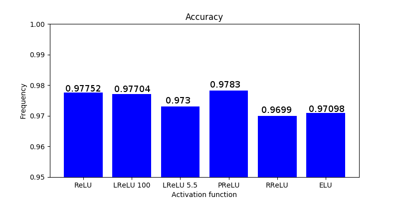
I coded the following simple network in Tensorflow, trained it on MNIST dataset and achieved a 0.984 accuracy:

2DConv [3,3,1,32]
2DConv [3,3,32,64]
Max pooling
Reshape to 12*12*64 = 9216
Dense 1,9216
Dense 9216,10

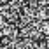
After this, the code was changed to only modify the network’s input and iterate 10 times (Note: the input did not significantly improved much after 10 iterations). The achieved result varies depending on the initial values of the input, as shown in the Table below.

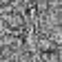
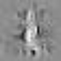
Table 1: The initial values to generate those images were the following: (first row, from left to right) ones, 0.5, (second row, from left to right) zeros and random

Although it may be difficult to see we can quickly understand that depending on the initial values our results will be significantly different, thus it is important to think and try different configurations. In spite of the results obtained from the randomly generated initial input, the other three present a similar structure: the center of the images have large values (white) and they are surrounded by negative values. You may have expected to reach results in which you can clearly see an horizontal white line surrounded by black pixels, but this trained network didn’t need that to distinguish between 1 and other classes. As we can see, the values in the center are the most significant.

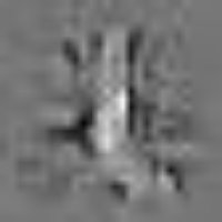
We may also see something similar in the random example. In this case, we can visualize the variation of the pixels comparing the initial with the final state.

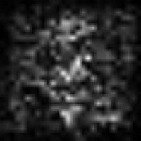
It is indeed hard to see. However, if you input the values obtained to generate this image into the classifier, you will get that the network classifies it as 1 with a 0.99999 confidence. For classifying a one, the network might not have to learn much about it.

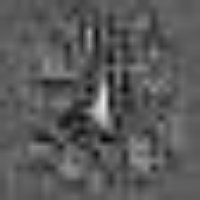
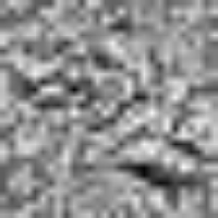
For this reason, I calculated the maximum variability between the 10 classes pixel-wise among the whole dataset (standard deviation) and concluded that the samples of the number 2 are very different among them. Let us try to see what would happen if we repeat the same experiment from a random initial state to maximize the activation function for a 2.

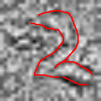
In this case, it is easier to see the number we want to classify. Again, using these values will provide with a right classification with a confidence of over 0.9999. In order to prove that the outer pixels (the first and last horizontal and vertical rows of pixels) are irrelevant, we can overwrite the values with 0 and still get a confidence of around 0.9989.

The code is provided in the Source code section.

Gradients in Tensorflow

June 9, 2018June 9, 2018 Juan Miguel Valverde Leave a comment

The chain rule in Tensorflow

Manipulating any type of neural network involves dealing with the backpropagation algorithm and thus it is key to understand concepts such as derivatives, chain rule, gradients, etc. It is often important to not only theoretically understand them but also being able to play around with them, and that is the goal of this post. Most of the information presented has been collected from different posts from stackoverflow.

There are three types of differentiation:

Numerical: it uses the definition of the derivative (lim) to approximate the result.
Symbolic: manipulation of mathematical expressions (the one we learn in high school).
Automatic: repeatedly using the chain rule to break down the expression and use simple rules to obtain the result.

As the author of the answer (Salvador Dali) in stackoverflow points out, symbolic and automatic differentiation look similar but they are different.

Tensorflow uses reverse mode automatic differentiation.

As mentioned above, Automatic differentiation uses the chain rule so there are two possible ways to apply it: from inside to outside (forward mode) and vice versa (reverse mode). In the Automatic differentiation Wikipedia page there are a couple of step-by-step examples of forward and reverse mode quite easy to follow. The reverse mode is a bit harder to see probably because of the notation introduced by the Wikipedia but someone made a simple decomposition easier to understand.

Gradients

Gradients of common mathematical operations are included in Tensorflow so they can be directly applied during the reverse mode automatic differentiation process. In fact, if you want to implement a new operation it has to inherit from Decop and its gradient has to be “registered” (RegisterGradient). For example, this is how the derivative of [latex s=2]f(x)=sin(x)[/latex] looks like (python/ops/math_grad.py):

@ops.RegisterGradient("Sin")
def _SinGrad(op, grad):
"""Returns grad * cos(x)."""
x = op.inputs[0]
with ops.control_dependencies([grad]):
x = math_ops.conj(x)
return grad * math_ops.cos(x)

The function tf.gradients is used by any optimizer because they all inherit from the class Optimizer (python/training/optimizer.py). tf.gradients is not commonly used directly but it is implicitly used when calling the function minimize as:

train_step = tf.train.GradientDescentOptimizer(learning_rate=0.01).minimize(loss)

More specifically, “minimize” function has two tasks:

Calculate gradients
Apply gradients

We can thus apply those operations, or even break down calculate_gradients to use tf.gradients. Here there are three alternatives when minimizing a loss function:

with tf.variable_scope("optimization") as scope:
optimizer = tf.train.GradientDescentOptimizer(learning_rate=0.01)
# Option 1:
train_step = optimizer.minimize(self.loss)
# Option 2:
grads = optimizer.compute_gradients(self.loss,var_list=tf.trainable_variables())
train_step = optimizer.apply_gradients(grads)
# Option 3:
grads = tf.gradients(loss,tf.trainable_variables())
grads_and_vars = list(zip(grads,tf.trainable_variables()))
train_step = optimizer.apply_gradients(grads_and_vars)

This decomposition of the function minimize can be useful in some cases. For instance, you may want to process or keep track of the gradients to understand the Graph computations or you may want to calculate the gradients with respect to only some variables and not all of them.

Simple tf.gradients example

We have the function [latex s=2]z = f(x,y) = 2x-y[/latex] and we want to calculate both of its partial derivatives [latex s=2]\frac{\partial z}{\partial x} = 2[/latex] and [latex s=2]\frac{\partial z}{\partial y} = -1[/latex].

import tensorflow as tf

x = tf.Variable(1)
y = tf.Variable(2)
z = tf.subtract(2*x, y)
grad = tf.gradients(z, [x, y])

sess = tf.Session()
sess.run(tf.global_variables_initializer())

res = sess.run(grad)
print(res) # [2, -1]

In the previous example we could not see that after the derivatives are calculated, tf.gradients also substitutes each variable by its value and performs the corresponding calculations. Another example: [latex s=2]z = f(x,y) = sin(x)-y^3[/latex]. [latex s=2]\frac{\partial z}{\partial x} = cos(x)[/latex], [latex s=2]\frac{\partial z}{\partial y} = -3y^2[/latex]

import tensorflow as tf

x = tf.Variable(3.)
y = tf.Variable(5.)

z = tf.subtract(tf.sin(x), tf.pow(y,3))
grad = tf.gradients(z, [x, y])
#upd = inp - tf.multiply(grad,0.01)
sess = tf.Session()
sess.run(tf.global_variables_initializer())

res = sess.run(grad)
print(res) # [-0.9899925, -75.0] <-> [cos(3), -3*5*5]

Dropout explained and implementation in Tensorflow

June 3, 2018June 3, 2018 Juan Miguel Valverde Leave a comment

Dropout

Dropout [1] is an incredibly popular method to combat overfitting in neural networks. The idea behind Dropout is to approximate an exponential number of models to combine them and predict the output. In machine learning it has been proven the good performance of combining different models to tackle a problem (i.e. AdaBoost), or combining models trained in different parts of the dataset. However, when it comes to deep learning, this becomes too expensive, and Dropout is a technique to approximate this.

Dropout can be easily implemented by randomly disconnecting some neurons of the network, resulting in what is called a “thinned” network. Thus, if the model has [latex]n[/latex] neurons, there are [latex]2^n[/latex] potential models. Each of them might be trained once or few times, or even not trained at all. Generating one of these random models is done batch-wise so in every batch there will be a new dropout mask (to disconnect the corresponding weights) generated. At train time, each neuron has a probably [latex]p[/latex] of being disconnected. For instance, if [latex]p=0.5[/latex] (recommended configuration, except for the input layer which is recommended to have [latex]p=0.8[/latex]) and we have 200 neurons, the first batch might encounter 90 activated neurons, the second batch might encounter 103 activated neurons, etc.

At test time, all neurons will multiply [latex]p[/latex].

In the image above we can see a simple implementation of a standard feedforward pass: weights multiply inputs, add bias, and pass it to the activation function. The second set of formulas describe how it would look like if we add dropout:

Generate a dropout mask: Bernoulli random variables (i.e. 1.0*(np.random.random((size))>p)
Apply the mask to the inputs disconnecting some neurons.
Use this new layer to multiply weights and add bias
Finally use the activation function.

All the weights are shared across the potential exponential number of networks, and during backpropagation, only the weights of the “thinned network” will be updated.

How is it implemented in Tensorflow?

In Tensorflow it is implemented in a different way that seems to be equivalent. Let’s have a look at the following example. According to the paper:

Let our neurons be: [latex][1,2,3,4,5,6,7,8][/latex] with [latex]p=0.5[/latex].
At train time, half of the neurons would be randomly disconnected, leading to [latex][1,0,0,4,5,0,7,0][/latex]
At test time, we would have multiplied the whole matrix by p, leading to [latex]0.5*[1,2,3,4,5,6,7,8][/latex]

In other words, we downgrade the outcome at testing time. In contrast, in Tensorflow, we do it the other way around. We increase the values at training time by [latex]1/prob[/latex]. Following our example:

Let our neurons be: [latex][1,2,3,4,5,6,7,8][/latex] with [latex]p=0.5[/latex].
At train time, half of the neurons are randomly disconnected, leading to [latex]1/0.5*[1,0,0,4,5,0,7,0] = [2,0,0,8,5,0,14,0][/latex]
At test time, we would use [latex]p=1[/latex], leading to [latex]1/1*[1,2,3,4,5,6,7,8][/latex]

In other words, at testing time we treat it as a normal neural network without dropout, and at training time we upscale the values by [latex]1/prob[/latex].

The reason why the values are upscale is to preserve the total sum (approx.).

[latex]sum([1,2,3,4,5,6,7,8]) = 36[/latex]
[latex]sum(1/0.5 * [1,0,0,4,5,0,7,0]) = 29[/latex]

This makes sense because if our layer produces certain output, we want to keep it approximately the same regardless of any method we are using to combat overfitting.

Dropout in Tensorflow

Adding a dropout layer in Tensorflow is really easy.

...
W = tf.get_variable("W",shape=[512,128],initializer=init)
b = tf.get_variable("b",initializer=tf.zeros([128]))

dropped = tf.nn.dropout(prev_layer,keep_prob=current_keep_prob)

dense = tf.matmul(dropped,W)+b
act = tf.nn.relu(dense)
...

Where current_keep_prob will be [latex]p[/latex] during training time and 1 during inference/testing time.

As I mentioned before, only those weights that were successfully masked (without the ones corresponding to the dropped out neurons) will be updated. If I have 100 neurons and [latex]p=0.5[/latex], half of the weights are expected to be updated. In the gif below we can see the evolution of 3 different plots: the first shows how the weights are being updated, the second shows which weights are being updated and the third is a cumulative sum of the second.

Optimizers comparison with and without Dropout

Due to the nature of AdamOptimizer, it does not follow this rule of updating only the weights belonging to the “thinned” network, so I found interesting to compare the performance of several optimizers in a simple neural network.

Test
Goal: To perform a first step to check the performance between Adam, Adadelta, Adagrad and Gradient Descent across different learning rates (1000 learning rates between 1e-6 to 1e-1).
Dataset: EMNIST (47 classes).
Batch size: 8.
Epochs: 1.
Network: conv2d (3,3,1,32), conv2d (3,3,32,64), max pooling (2,2), reshape (12*12*64), dense (12*12*64,128), dense (128,47).
Weights initialization: he_uniform. Bias initialization: zeros.
Activation layers: ReLU (and softmax at the end of the network).
Cost function: cross entropy.

These graph does not show the actual performance of dropout under each optimizer since I only tested a bunch of learning rates without properly examine and focus where it seems to provide good results. In addition, it is not fair to compare on the same learning rates dropout vs non-dropout. Instead, this shows how a first step looks like .

References

1. NNitish Srivastava, Geoffrey Hinton, Alex Krizhevsky, Ilya Sutskever, Ruslan Salakhutdinov. 2014. “Dropout: A simple way to prevent neural networks from overfitting”

Image style transfer using convolutional neural networks – Tensorflow implementation

April 24, 2018April 24, 2018 Juan Miguel Valverde Leave a comment

Recently I recorded a video explaining in a very simple way how style transfer works in a convolutional neural network (VGG16) based on the incredibly well-written paper by Gatys et al [1]. I also implemented it in an extremely concise and simple way (around than 150 lines with comments).

Original Image

Combinations

The code is provided in the Source code section.

References

1. Gatys LA, Ecker AS and Bethge M. 2016. Image Style Transfer Using Convolutional Neural Network.

Difference between L1 and L2 regularization, implementation and visualization in Tensorflow

January 19, 2018January 19, 2018 Juan Miguel Valverde Leave a comment

Regularization is a technique used in Machine Learning to penalize complex models. The reason why regularization is useful is because simple models generalize better and are less prone to overfitting.

Examples of regularization:

K-means: limiting the splits to avoid redundant classes
Random forests: limiting the tree depth, limiting new features (branches)
Neural networks: limiting the model complexity (weights)

In Deep Learning there are two well-known regularization techniques: L1 and L2 regularization. Both add a penalty to the cost based on the model complexity, so instead of calculating the cost by simply using a loss function, there will be an additional element (called “regularization term”) that will be added in order to penalize complex models.

The theory

L1 regularization (LASSO regression) produces sparse matrices. Sparse matrices are zero-matrices in which some elements are ones (the sparsity refers to the ones), but in this context a sparse matrix could be several close-to-zero values and other larger values. From the data science point of view this is interesting because we can reduce the amount of features. If we find a model with neurons whose weights are close to zero it means we don’t need those neurons because the model deactivates them with zeros and we might not need a specific feature/input leading to a simpler model. For instance, if we have 50 coefficients but only 10 are non-zero, the other 40 are irrelevant to make our predictions. This is not only interesting from the efficiency point of view but also from the economic point of view: gathering data and extracting its features might be a very expensive task (in terms of time and money). Reducing this will benefit us.

Due to the absolute value, L1 regularization provides with a non-differentiable term, but despite of that, there are methods to minimize it. As we will see below, L1 regularization is also robust to outliers.

L2 regularization (Ridge regression) on the other hand leads to a balanced minimization of the weights. Since L2 uses squares, it emphasizes the errors, and it can be a problem when there are outliers in the data. Unlike L1, L2 has an analytical solution which makes it computationally efficient.

Both regularizations have a λ parameter which is directly proportional to the penalty: the larger λ the stronger penalty to find complex models and it will be more likely that the model will avoid them. Likewise, if λ is zero, regularization is deactivated.

The graphs above show how the functions used in L1 and L2 regularization look like. The penalty in both cases is zero in the center of the plot, but this also implies that the weights are zero and the model will not work. The values of the weights try to be as low as possible to minimize this function, but inevitably they will leave the center and will head outside. In case of L2 regularization, going towards any direction is okay because, as we can see in the plot, the function increases equally in all directions. Thus, L2 regularization mainly focuses on keeping the weights as low as possible.

In contrast, L1 regularization’s shape is diamond-like and the weights are lower in the corners of the diamond. These corners show where one of the axis/feature is zero thus leading to sparse matrices. Note how the shapes of the functions shows their differentiability: L2 is smooth and differentiable and L1 is sharp and non-differentiable.

In few words, L2 will aim to find small weight values whereas L1 could put all the values in a single feature.

L1 and L2 regularization methods are also combined in what is called elastic net regularization.

The practice

One of my motivations to try this out was an “intuitive explanation” of L1 vs. L2 I found in quora.

From the theoretical point of view it makes sense: L2 emphasizes errors due to the square, and it will try to minimize them all of them equally so the line will get a bit off from the main trend because a big errors influences more than small errors. On the other hand, for L1 errors have the same importance (linearly speaking) so it will minimize a lot of errors getting really close to the main train even if there are outliers.

I created a small dataset of samples that describes a straight line and I later added noise and some outliers. I created a model with more neurons than needed to solve this problem in order to see whether it works and compare the weight evolution between the methods.

Model characteristics:
-Layers: 1 input, 3 hidden, 1 output
-Sizes: 1,10,10,10,1
-Batch size: 1 (noiser)
-Optimizer: SGD (lr=0.01)
-Lambda: 0.3 (for regularization)

I run the model 5 times with each regularization method and these are the results.

When the random outliers are sufficiently far none of them present good results, but overall the results obtained with L2 performance were better than those obtained with L1. Then, I had a look at the weights. Below, I show the weights and the results obtained with an additional run of the model.

As expected, L1 generates several 0-weighted neurons, so the model doesn’t use them. In other experiments, I got that most of the neurons were disconnected and only few of them had non-zero weights. On the other hand, L2 minimizes the values of the weights until most of them have a very low value.

Adjusting the network according to L1

As described before, L1 generates sparse matrices with disconnected neurons. If a neuron is disconnected, we don’t need it, leading to simpler models. I run again the script that uses L1 and I will adjust the model using less neurons according to the neurons it disconnects. Using the same samples and running the model 5 times, I got this total errors: 22.68515524, 41.64545712, 4.77383674, 24.04390211, 7.25596004.

The weights in this first run look like this:

I adjusted the neurons of the model: From [(1,10),(10,10),(10,10),(10,1)] to [(1,10),(10,10),(10,1),(1,1)] and this are the weights (note: the last big square is a single weight):

Performance on 5 runs: 7.61984439, 13.85177842, 11.95983347, 16.95491162, 25.17294774.

Implementation in Tensorflow

Despite the code is provided in the Code page as usual, implementing L1 and L2 takes very few lines: 1) Add regularization to the Weights variables (remember the regularizer returns a value based on the weights), 2) collect all the regularization losses, and 3) add to the loss function to make the cost larger.

with tf.variable_scope("dense1") as scope:
W = tf.get_variable("W",shape=[1,10],initializer=tf.contrib.layers.xavier_initializer(),regularizer=tf.contrib.layers.l2_regularizer(lambdaReg))
...
reg_losses = tf.reduce_sum(tf.get_collection(tf.GraphKeys.REGULARIZATION_LOSSES))
cost = tf.reduce_sum(tf.abs(tf.subtract(pred, y)))+reg_losses

Conclusion

The performance of the model depends so much on other parameters, especially learning rate and epochs, and of course the number of hidden layers. Using a not-so good model, I compared L1 and L2 performance, and L2 scores were overall better than L1, although L1 has the interesting property of generating sparse matrices.

Hypothetical improvements: This post aimed to show in a very simple and graphic/animated way the effects of L1 and L2. Further research would imply trying more complex models with data that gives stable results. After tunning the parameters to get the best results, one could use cross validation to compare better the performance.

The code is provided in the Source code section.

How to freeze a graph in Tensorflow

January 15, 2018February 7, 2018 Juan Miguel Valverde Leave a comment

I run into this issue when I was interested in freezing graphs for using them in mobile devices. Freezing a Graph means combining the structure of a model with its weights, so first we need to save those two parts to later combine them.

Saving the structure

# "g" will be your Graph
g = sess.graph
# In my case, I use the default Graph
gdef = g.as_graph_def()
# Parameters: 1) graph, 2) directory where we want to save the pb file,
# 3) name of the file, 4) text format (True) or binary format.
tf.train.write_graph(gdef,".","graph.pb",False)

Note: if we save our graph as text, setting the boolean value to True, we can have a look at it with any text editor and see how it looks like. Since it uses Protocol Buffers it is easily readable.

Saving the weights

We also call this the checkpoints. We have to get a Saver object and use it after the network is trained so it will contained the weights obtained after the optimization.

# When defining the model
saver = tf.train.Saver()
# ....
# After the model is trained
saver.save(sess, 'tmp/my-weights')

Freezing the Graph

Now it’s time to combine both files. We can see the commands in the original tutorial in github.

Since I didn’t want to mess up with my current tensorflow library, I downloaded tensorflow again in a separate folder

git clone https://github.com/tensorflow/tensorflow.git

After I installed Bazel (following their website instructions) I tried to build the freeze_graph (make sure you are in the right path. If you download again tensorflow from github note that it has a “WORKSPACE” file. You should be there to run Bazel) by doing:

bazel build tensorflow/python/tools:freeze_graph

It takes a while to build it. In MacOS Sierra I didn’t have any problem, but in Ubuntu 16.04 I did, and after searching I found on github how to solve it.

bazel build -c opt --copt=-msse4.1 --copt=-msse4.2 tensorflow/python/tools:freeze_graph

After this, in the same folder, we just need to execute the command provided in the tutorial:

bazel-bin/tensorflow/python/tools/freeze_graph\
--input_graph=/tmp/mobilenet_v1_224.pb \
--input_checkpoint=/tmp/checkpoints/mobilenet-10202.ckpt \
--input_binary=true --output_graph=/tmp/frozen_mobilenet_v1_224.pb \
--output_node_names=MobileNet/Predictions/Reshape_1

input_graph: location of the structure of the graph (first part of the tutorial, pb file)
input_checkpoint: weights stored using the Saver (second part of the tutorial)
input_binary=true: remember to save the graph in binary format. They recommend that this value has to be true, so do not use text format generating the pb file.
output_graph: location of the new frozen graph
output_node_names: name of the output node. You can check this using Tensorboard, but assuming you are naming all the tensors, this should be easy to figure out. You can also check the name of all the operations, or check the pb file (text mode), but probably the most intuitive way is using Tensorboard.

After executing this, we will have our frozen graph.

Bonus: How to use the frozen Graph in Python

Here I found a very easy to follow code that explains itself how to read a frozen Graph to use it.

import tensorflow as tf

def load_graph(frozen_graph_filename):
# We load the protobuf file from the disk and parse it to retrieve the
# unserialized graph_def
with tf.gfile.GFile(frozen_graph_filename, "rb") as f:
graph_def = tf.GraphDef()
graph_def.ParseFromString(f.read())

# Then, we import the graph_def into a new Graph and returns it
with tf.Graph().as_default() as graph:
# The name var will prefix every op/nodes in your graph
# Since we load everything in a new graph, this is not needed
tf.import_graph_def(graph_def, name="prefix")
return graph

Colorizing black and white images using Deep Learning (Tensorflow)

September 26, 2017January 19, 2018 Juan Miguel Valverde Leave a comment

Recently I was reading up on an interesting paper that explores how colorizing black and white images using Deep Learning. The paper was easy to read and understand, and to fully enjoy it I decided to implement it in a lower scale. I have a laptop with a humble graphic card and an i7 so it cannot compete with those servers that cost several thousand euros, that is why I have not focused on the design of the network but more on the algorithmic part.

Goals and dataset

The goals of this post are:

To be able to implement the algorithm to learn about a new colorizing approach.
To have a look to the neural network they used.
To figure out if a simpler network can learn even if the results are quite improvable.
To practice using tensorflow.
To have fun.

The dataset I will use can be downloaded here. It consist of 2687 256×256 images of beaches, forests, streets, etc.

Algorithm

One of the things I enjoyed about the paper [1] is how well structured it is, which made the understanding much easier. I will try to follow their structure in a similar way while being precise and concise.

The very first important thing we need to know is that Lab color space is used. The reason is simple: in color spaces such as RGB we need to learn three different channels whereas in Lab we only need to learn two. The channel L refers to the lightness, having values between 0 (dark) and 100. The channels a and b are the position in the axis between red-green and blue-yellow respectively.

A typical approach would use the L channel as input and the a,b channels as output (for every pixel the prediction consists on two values). However, they argue that using a loss function based on two components does not represent the multimodal and ambiguity problems properly. We are surrounded by objects that can have multiple colors such as apples since they can be red, green or yellow. In addition, Euclidian distance (averaging) will increase desaturated (grayish) values.

In order to solve this they divided the a,b colorspace into Q bins corresponding to probabilities, and consequently, the number of predictions expected per pixel will be Q (one per bin). For instance, in case of the apple, the bins corresponding to red, yellow and green will contain higher probabilities than those bins close to colors like blue.

I skipped representing some bins by analyzing first the colors I have in my dataset so that I only take into account those bins with colors used in my dataset. My a,b color space is between -110 and 110 and depending on the size of the squared window used to divide it, the resulting grid and the final used bins will be different. When I’m using the whole dataset and a window size of 10 I use XX bins and it raises to XXX bins when the window size is 5. In contrast, the authors use Q=313 bins.

The problem is now a simple classification problem in which we have an input (brightness values) and the output is a set of probabilities indicating how likely are the values to belong to a certain bin. A classic way to solve this is to use cross entropy but in addition to it, the authors noticed that the model is biased towards low a,b values which typically correspond to backgrounds such as walls, sky, etc. In order to solve this, they rebalanced the colors by adding weights that will multiply the cross entropy calculated.

This formula can be read as: perform cross-entropy on a pixel comparing the original and predicted distribution of the probabilities, and then multiply it by a weight corresponding to that color such that certain colors are highlighted to the network.

To calculate these weights they introduced a new hyper-parameter [latex]\lambda[/latex] (they use [latex]\lambda=0.5[/latex]). Q was the number of bins used and [latex]\tilde{p}[/latex] is a distribution calculated from our dataset. I tried to use the full dataset consisting of different types of images and another consisting only of images of forests so I had to recalculated it. You can count the number of pixels that are located within each bin and later normalize it. They also apply a Gaussian kernel but I actually skipped that part. The image below depicts which colors are used the most in the dataset.

In the image above, the left side shows that the most used colors are located in the center (desaturated) and both cases differ depending on the dataset: when only forest images were used, less pink-red colors were used.

This is basically all, in regards to the training part. The other important issue arises when predicting values. Imagine for a second that for a single pixel the network spits a probability distribution such that all values are zero except for one value that is one (the so called one-hot vector). It is more than clear that the corresponding bin will represent the color of that pixel. Nonetheless, we will probably have several probabilities and mapping them back to a,b values is the next task. They introduced a new variable called T standing for temperature (coming from simulated annealing). To put it simple, when T tends to zero, values are more intense since the prediction emphasizes the color with the highest probability. On the other hand, when T tends to one, the colors are more distributed but also more desaturated because the color is result of a more spread average of the obtained probabilities.

The formula above describes how they calculated the prediction given the temperature T and the distribution z.

Neural Network

As I have mentioned before, due to my limited resources, utilizing the network they used was immediately discarded. Thus I designed a very simple neural network that consists of 8 convolutional layers. The input consist of a window of 32×32 pixels and after the convolutions the final prediction has a size of 16×16. In every convolution the size is reduced by 2 because of the 3×3 kernel thus reducing one pixel on each side of the image. The number of filters used depends on the number of bins Q such that they are growing using a step of Q/8. For instance, the number of filters in the first convolutional layer is Q/8, in the second layer is 2*Q/8, and so on until the last layer with a number of Q filters. Therefore, the size of my final output will be 16x16xQ.

Results

At first I was using only the forest dataset to speed up the training process and regardless of some hyper-parameters tunning the results were a bit random: sometimes they were quite okay and sometimes they were bad, but in all cases the network was learning and showing a behavior that makes sense, so I can say that I am satisfied with the results.

The code is provided in the Source code section.

References

1. Zhang R., Isola P. & Efros A.A. 2016. Colorful Image Colorization.

Informal review on Randomized Leaky ReLU (RReLU) in Tensorflow

September 1, 2017September 1, 2017 Juan Miguel Valverde Leave a comment

This very informal review of the activation function RReLU compares the performance of the same network (with and without batch normalization) using different activation functions: ReLU, LReLU, PReLU, ELU and an less famous RReLU. The difference between them lies on their behavior from [latex][- \infty,0][/latex]. The goal of this entry is not to explain in detail these activation functions, but to provide a short description.

When a negative value arises, ReLU deactivates the neuron by setting a 0 value whereas LReLU, PReLU and RReLU allow a small negative value. In contrast, ELU has a smooth curve around the zero to make it derivable resulting in a more natural gradient and instead of deactivating the neuron negative values are mapped into a negative one. The authors claim that this pushes the mean unit closer to zero, like batch normalization [1].

LReLU, PReLU and RReLU provide with negative values in the negative part of the respective functions. LReLU is using a small tilted slope whereas PReLU learns the steepness of this slope. On the other hand, RReLU, the function we will study here, sets this slope to be a random value between an upper and lower bound during the training and an average of these bounds during the testing. The authors of the original paper get their inspiration from Kaggle competition and even use the same values [2]. These are random values between 3 and 8 during the training and a fixed value 5.5 during testing.

Notice that in [2] and consequently in the following tests, the variable [latex]\alpha_i[/latex] that uses LReLU is not used as [latex]\alpha_i x_i[/latex] but as [latex]\frac{x_i}{\alpha_i}[/latex]. This detail is important and for some reasons [2] change the notation from the original LReLU paper.

Results

As in the paper where RReLU is introduced, I used the same activation function configurations plus ELU (default configuration). I run a very simple neural network using MNIST dataset with and without batch normalization and as we can see in the figure below RReLU does not only perform among the words but the simple ReLU performs the best when normalization is used and almost the best when no normalization is added.

Notes on Tensorflow

This activation function requires to constantly use new random values that need to be initalized constantly while the network is training. As we can see in the corresponding tutorial video and the source code the initializer needs to be called on each iteration during the training by:

sess.run(r1.initializer)

The code is provided in the Source code section.

References

1. Clevert D.A., Unterthiner T. and Hochreiter S. 2016. Fast and accurate Deep Network Learning by Exponential Linear Units (ELUs). ICLR 2016.
2. Xu B., Wang N., Chen T. and Li M. 2015. Empirical Evaluation of Rectified Activations in Convolutional Network.

Tensorflow Video tutorial

August 19, 2017January 6, 2018 Juan Miguel Valverde 4 Comments

Since I have free time I would like to record some videos showing how to use Tensorflow.

Tensorflow Tutorial 1 – A very simple Neural Network
Source code: https://github.com/jmlipman/LAID/blob/master/Tensorflow/Tutorial/1_nn.py

Tensorflow Tutorial 2 – A very simple Convolutional Neural Network
Source code: https://github.com/jmlipman/LAID/blob/master/Tensorflow/Tutorial/2_cnn.py

Tensorflow Tutorial 3 – Encapsulating CNN’s code with get_variable and variable_scope
Source code: https://github.com/jmlipman/LAID/blob/master/Tensorflow/Tutorial/3_cnn_pretty.py

Tensorflow Tutorial 4 – Batch Normalization
Source code: https://github.com/jmlipman/LAID/blob/master/Tensorflow/Tutorial/4_batchNormalization.py

Tensorflow Tutorial 5 – Customized activation function, RReLU
Source code: https://github.com/jmlipman/LAID/blob/master/Tensorflow/Tutorial/5_customizedActivationRReLU.py

Tensorflow Tutorial 6 – Autoencoder
Source code: https://github.com/jmlipman/LAID/blob/master/Tensorflow/Tutorial/6_autoencoder.py