Category: Papers

Title: U-Net Convolutional Networks for Biomedical Image Segmentation
Authors: Olaf Ronneberger, Philipp Fischer, Thomas Brox
Link: https://arxiv.org/abs/1505.04597

Quick Summary:

One of the interesting things about the paper is the architecture used. They share they weights of the “contracting path” in the “expansive path”, and since the sizes are different, they are forced to crop them (blue dots in the layers).

One of the challenges faced by the authors were the separation between different cells that belong to the same class. For this, they propose using a weighted loss where those separations have a large weight in the loss function.

Training uses a high momentum (0.99) because they don’t have many training samples. Thus, a large number of the previously seen training samples determine the update of the current optimization step. In addition, they perform data augmentation for the model to be rotation and shift invariant, and robust to deformations and gray value variations.

Title: Confidence Estimation in Deep Neural Networks via Density Modelling
Authors: Akshayvarun Subramanya, Suraj Srinivas, R.Venkatesh Babu
Link: https://arxiv.org/abs/1707.07013

Quick Summary:
Confidence level via traditional softmax activation function does not produce very good estimates. Given an input, if we increase its values (for instance, x1.3), the confidence of the winner class will consequently increase.

The authors propose to estimate the confidence level based on density modelling. Given our inputs [latex]X[/latex] and the pre-softmax result [latex]z[/latex], and since there is one-to-one mapping from [latex]X[/latex] to [latex]z[/latex], we are interested in calculate [latex]P(y_i | X)[/latex] (probability of each class given the input X).

[latex]P(y_i | z) = \frac{P(z | y_i) P(y_i)}{\sum_{j=1}^N P(z | y_i) P(y_i)}[/latex]

[latex]P(y_i)[/latex]: probability of having that class.
[latex]P(X | y_i) = N(z | \mu_i, \sigma_i)[/latex]: the probability is the value [latex]z[/latex] of the normal distribution of [latex]\mu_i, \sigma_i[/latex]. The mean and variance are learn during the training and the density function is generated.

A more graphical and probably easy-to-understand way to see this is to think that we have a vector [latex]z[/latex] of size N (number of classes). To get the confidence level we would normally use a softmax function, but instead, the authors calculate a density model to calculate later how likely is that given a specific [latex]z[/latex], we predict [latex]y_i[/latex].

Title: On Calibration of Modern Neural Networks
Authors: Chuan Guo, Geoff Pleiss, Yu Sun, Kilian Q. Weinberger
Link: https://arxiv.org/abs/1706.04599

Quick Summary:
A model is considered calibrated if their confidence levels (probabilities) and their predictions are correlated. For instance, if we predict Y with a confidence level of 0.7, we expect that it will be right the 70% of the times. In contrast, if our model have predictions whose confidence is around 0.9 but they are right only about half of the times (50%) the model is not well calibrated.

The authors describe that recent models are often non-calibrated. The provide some measures to calculate the miscalibration (Expected Calibration Error and Maximum Calibration Error). ECE can be useful in a general application whereas MCE is useful in high-risk applications where we need to be very confident to perform an action (diagnosis prediction). Miscalibration often comes in models with high capacities (deep and wide) and lack of regularization.

There is no correlation between miscalibration and accuracy. They argue that a model can overfit its loss while getting better at predictions. One of their conclusions is “the network learns better classification accuracy at the expense of well-modeled probabilities”.

The authors mention some calibration methods. For binary models: histogram binning, isotonic regression, bayesian binning into quantiles and platt scaling. For multiclass models: extension of binning methods, matrix and vector scaling and temperature scaling. The one who seems to work better is “temperature scaling”.

Temperature scaling can soften the softmax, so if we do [latex]z_i/T[/latex] the model can be more calibrated. Temperature scaling won’t change the element of the vector [latex]z_i[/latex] that has the maximum value, so the accuracy won’t be affected at all. Personal note: this is linked to another paper I’m reading which indeed mentions that upscaling the values of [latex]z_i[/latex] distorts the confidence levels making the maximum value increase.

The authors conclude with “modern neural networks exhibit a strange phenomenon: probabilistic error and miscalibration worsen even as classification error is reduced”.

Title: Maxout Networks
Authors: Ian J. Goodfellow, David Warde-Farley, Mehdi Mirza, Aaron Courville, Yoshua Bengio
Link: https://arxiv.org/abs/1302.4389

Quick summary:
Maxout is an activation function that takes the maximum value of a bunch of neurons. In one sense, one could think as dropout being similar since dropout will discard some neurons and will pass forward others whereas maxout will only pass the maximum value of some of them. In essence, maxout is like max pooling since it reduces the dimensionality leaving only the maximum values.

It is well explained in the following post: http://www.simon-hohberg.de/blog/2015-07-19-maxout
Goodfellow PhD’s defence (talking about maxout): https://www.youtube.com/watch?v=ckoD_bE8Bhs&t=28m

Nowadays it is also implemented in tf.contrib.layers.maxout but here is a very simple implementation:

Title: Large-batch training for Deep Learning: Generalization gap and Minima
Authors: Nitish Shirish Keskar, Dheevatsa Mudigere, Jorge Nocedal, Mikhail Smelyanskiy, Ping Tak Peter Tang
Link: https://arxiv.org/abs/1609.04836

Quick summary:
The main goal of this paper is to discuss about the minimizers resulting from using large and small batch size and to provide with a measure of how sharp is the minimum found. Loss functions depend on both the geometry of the cost function and the size and properties of the training set. Using batches have been proven to converge to minimizers and stationary points of strongly-convex functions, avoid saddle-points and robustness to input data, but a large batch size is shown to lead to a loss in generalization performance (generalization gap).

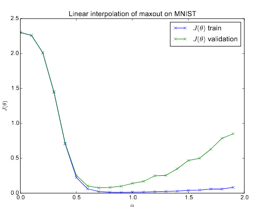
They observe that this loss of generalization is related to the sharpness of the minimizer obtain by large-batch (LB) methods. On the other hand, methods using small batch (SB) lead to flatter minimizers.

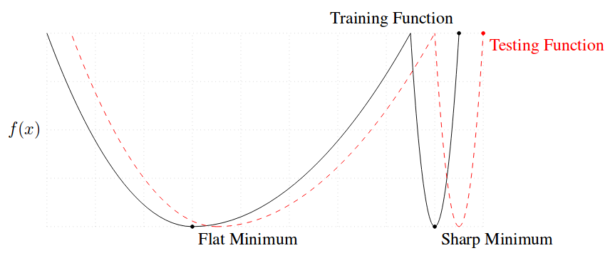
There is a clear trade-off because LB are desirable since they are computationally efficient and less noisy but if they are too large they will not generalize well. They mention some reasons why this might happen: 1) LB methods produce overfitting, 2) they are attracted to saddle points, 3) they lack the exploratory properties SB has, 4) and they tend to zoom-in on the minimizer closest to the initial point. They had a look at the minimizers and realized that sharp minimizers have significantly large positive eigenvalues whereas flat minimizers have small eigenvalues, thus their conclusion is that the sharpness of a minimizer can be characterized by the magnitude of the eigenvalues [latex]\nabla^2 f(x)[/latex].

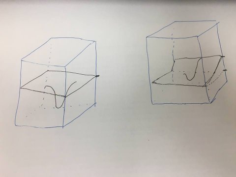
For this reason, they come up with a formula to measure the sharpness of a function, and the results show that it can distinguish quite well how different it is the minimizer when large and small batches are used. This measure is basically based on drawing a small box around the minimizer and check largest value. However, a minimizer does not usually have the shape of a cone. Values at one side can be very large whereas on the other side be flatter.

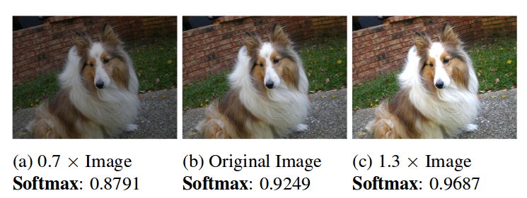
They try to improve the generalization problem of LB by doing data augmentation, conservative training and adversarial training and although they help to reduce the generalization gap, they do not solve the problem completely. They also experiment combining small and large batches and hypothesize that a gradual increase of the batch size might help the generalization process.

The authors observe that the noisy in the gradient when using SB pushes the iterates out of sharp minimizers, thus encouraging movement towards a flatter minimizer. They also observe that LB methods are usually attracted to minimizers close to the starting point and, in contrast, SB tend to go further away.

Title: Qualitatively characterizing neural network optimization problems
Authors: Ian J. Goodfellow, Oriol Vinyals, Andrew M. Saxe
Link: https://arxiv.org/abs/1412.6544

Quick Summary:
The main goal of the paper is to introduce a simple way to look at the trajectory of the weights optimization. They also mention that it might be possible that some NN are difficult to train due to the effect of their complex structures in the cost function or the noisy introduced in the minibatches because they didn’t find that local minima and saddle points slow down the SGD learning.

This technique consist in evaluating [latex]J(\theta)[/latex] (the cost function) where [latex]\theta = (1-\alpha) \theta_0 + \alpha \theta_1[/latex] for different values of [latex]\alpha[/latex]. They set [latex]\theta_0 = \theta_i[/latex] (initial weights) and [latex]\theta_1 = \theta_f[/latex] (weights after training), and we can get a cross-section of the objective function.

We can see thus whether there are some bumps or flats during the training given the training/testing data. They do not mention if they averaged the costs obtained with the training and testing datasets, but I guess so because otherwise they would be significantly different.