Introduction to Activation Maximization and implementation in Tensorflow

June 18, 2018June 18, 2018 Juan Miguel Valverde Leave a comment

Introduction

The goal of this entry is to learn about activation maximization and to prove two basic well-known facts about Deep Learning.

The way a NN learns the representation of something does not neet to be in a significant way for humans. In fact, most of the times it’s not.
The found minima depends (among other factors) on the initial state.

It might be interesting to have a look at the representation the NN creates of a object (in case of classification) in order to understand why it is [not] performing well. To make it simple, I used MNIST dataset to create a NN capable of recognizing 0-9 digits. If we think of how does a 1 need to look like so that a person can understand it is a 1, we may think of it as a vertical straight line that can be a bit tilt.

Activation Maximization

Activation maximization, as the name indicates, aims to maximize the activation of certain neurons. Imagine you are training your model with a single image several times. Training is changing the weights accordingly to achieve the lowest loss possible, so the input and the desired output will be constant whereas the weights will be modified iteratively until we reach a minima (or until we decide to stop training). In Activation Maximization, we will keep the weights and the desired output constant and we will modify the input such that it maximizes certain neurons.

I coded the following simple network in Tensorflow, trained it on MNIST dataset and achieved a 0.984 accuracy:

2DConv [3,3,1,32]
2DConv [3,3,32,64]
Max pooling
Reshape to 12*12*64 = 9216
Dense 1,9216
Dense 9216,10

After this, the code was changed to only modify the network’s input and iterate 10 times (Note: the input did not significantly improved much after 10 iterations). The achieved result varies depending on the initial values of the input, as shown in the Table below.

Table 1: The initial values to generate those images were the following: (first row, from left to right) ones, 0.5, (second row, from left to right) zeros and random

Although it may be difficult to see we can quickly understand that depending on the initial values our results will be significantly different, thus it is important to think and try different configurations. In spite of the results obtained from the randomly generated initial input, the other three present a similar structure: the center of the images have large values (white) and they are surrounded by negative values. You may have expected to reach results in which you can clearly see an horizontal white line surrounded by black pixels, but this trained network didn’t need that to distinguish between 1 and other classes. As we can see, the values in the center are the most significant.

We may also see something similar in the random example. In this case, we can visualize the variation of the pixels comparing the initial with the final state.

It is indeed hard to see. However, if you input the values obtained to generate this image into the classifier, you will get that the network classifies it as 1 with a 0.99999 confidence. For classifying a one, the network might not have to learn much about it.

For this reason, I calculated the maximum variability between the 10 classes pixel-wise among the whole dataset (standard deviation) and concluded that the samples of the number 2 are very different among them. Let us try to see what would happen if we repeat the same experiment from a random initial state to maximize the activation function for a 2.

In this case, it is easier to see the number we want to classify. Again, using these values will provide with a right classification with a confidence of over 0.9999. In order to prove that the outer pixels (the first and last horizontal and vertical rows of pixels) are irrelevant, we can overwrite the values with 0 and still get a confidence of around 0.9989.

The code is provided in the Source code section.

[Neural Networks] Multilayer Perceptron

June 3, 2015February 5, 2017 Juan Miguel Valverde Leave a comment

Definition

An MLP (Multilayer perceptron) is a feedforward neural network which consists of many perceptrons joined in many layers. The most basic MLP has 3 layers: one input layer, one output layer and one hidden layer, but it may have as many hidden layers as necessary. Each individual layer may contain a different number of neurons.

[latex]
W_1 = \begin{bmatrix}
a & b & c \\
d & e & f \\
g & h & i
\end{bmatrix}

\quad

W_2 = \begin{bmatrix}
.. & .. & .. & ..
\end{bmatrix}
[/latex]

Feedforward means that nodes have a direct connection such that nodes located in between are fed by the outputs of previous nodes and so on. This is very simple to program because it is basically as the perceptron: multiply weights (including bias nodes) by the input vector, give the result to the activation function, and the output will be the input of the next layer until the output layer is reached.

In the entry about the perceptron I used the step function as the activation function, but in MLP a variety of them can be used. Most of them are sigmoid (mathematical functions having an “S” shape) such as:

The difference between these two sigmoids is that the hyperbolic tangent goes from -1 to 1 whereas the other goes from 0 to 1.

Sometimes linear functions are also needed for cases when neural networks are not used for classification but for extrapolation and any kind of prediction.

If the MLP misclassifies an input, it is necessary to back-propagate the error rate through the neural network in order to update old weights. Gradient descent through derivatives is used to correct the weights as much as possible. Derivatives show how the error varies depending on the weights to later apply the proper correction.

In perceptrons, the error function was basically [latex]t_i – y_i[/latex] (desired output minus system’s output) but in MLP the squared error function will be used instead [latex]J = \sum \frac{1}{2}(y-\widehat{y})^2[/latex]:

It has a sum because each element has its own error and it is necessary to sum them up.
It is squared because convex functions’ local and global minima are the same.
It has a [latex]\frac{1}{2}[/latex] to make it simpler when obtaining the derivative.

The following mathematical explanation regarding the formulas for the learning process is based on the 2x3x1 neural network depicted in the first picture of the entry, but before that, some terms need to be introduced to avoid misunderstandings:

[latex]X \to [/latex] Input matrix.
[latex]W_1 \to [/latex] Weights’ matrix that connects the input and hidden layers.
[latex]W_2 \to [/latex] Weights’ matrix that connects the hidden and output layers.
[latex]y \to [/latex] Desired output.
[latex]\eta \to [/latex] Learning rate.
[latex]z_2 = x*W_1 \to [/latex] Content of each node in the hidden layer (before activation).
[latex]a_2 = f(z_2) \to [/latex] Content of each node in the hidden layer (after activation).
[latex]z_3 = a_2*W_2 \to [/latex] Content of each node in the output layer (before activation).
[latex]\widehat{y} = f(z_3) \to [/latex] MLP output.
[latex]J = \sum \frac{1}{2}(y-\widehat{y})^2 \to [/latex] Squared error function.

First, let us calculate the update formula for [latex]W_2[/latex]. For this, it is necessary to calculate the derivative of the error with respect to [latex]W_2[/latex] to see how much the error varies depending on [latex]W_2[/latex].

[latex]\frac{\partial J}{\partial W_2} = \frac{\partial \sum \frac{1}{2} (y – \widehat{y})^2}{\partial W_2} = \sum \frac{\partial \frac{1}{2} (y – \widehat{y})^2}{\partial W_2}
[/latex]

By the sum rule in differentiation we can take the sum off the fraction, and from now on it is no longer needed since at the end we can sum each sample individually, so let us derive it.

[latex]\frac{1}{2} \cdot 2 \cdot (y – \widehat{y}) \cdot [ \frac{\partial y}{\partial W_2} – \frac{\partial \widehat{y}}{\partial W_2} ][/latex]

The derivative of y with respect to [latex]W_2[/latex] is 0 since y does not depend on [latex]W_2[/latex].

[latex]-1 (y – \widehat{y}) \cdot \frac{\partial \widehat{y}}{\partial W_2}[/latex]

By applying the chain rule:

[latex]-1 (y – \widehat{y}) \cdot \frac{\partial \widehat{y}}{\partial z_3} \cdot \frac{\partial z_3}{\partial W_2}[/latex]

Which finally:

[latex]-1 (y – \widehat{y}) f'(z_3) \cdot a_2 \to \delta_3[/latex]

In case of [latex]W_1[/latex] the procedure is very similar:

[latex]\frac{\partial J}{W_1} = [\text{same things…} ] = \delta_3 \cdot \frac{\partial z_3}{\partial W_1} = \delta_3 \cdot \frac{\partial z_3}{\partial a_2} \cdot \frac{\partial a_2}{\partial W_1} \\
= \delta_3 \cdot W_2 \cdot \frac{\partial a_2}{\partial z_2} \cdot \frac{\partial z_2}{\partial W_1} = \delta_3 \cdot W_2 \cdot f'(z_2) \cdot x[/latex]

Learning process (update rules):
[latex]W_1 = W_1 + \eta \frac{\partial J}{\partial W_1} \\
W_2 = W_2 + \eta \frac{\partial J}{\partial W_2}[/latex]

Results

The MLP I developed was able to correctly classify samples from its training set from 3 different classes. I have not written a word about overfitting because I will probably do that in a different entry with a good solution to overcome it, but this algorithm probably overfits and cannot classify other samples with the same good result.

Finally, I recorded the evolution of the error with two different learning rate to show that if [latex]\eta[/latex] is too big, it can escape from the minimum with an unknown result. In this case, it resulted absolutely good, but it is not always the case.

Left: [latex]\eta = -0.2[/latex]. Right: [latex]\eta = -0.1[/latex]

The code is provided in the Source code section.

References

I strongly recommend the set of videos to which this one belongs to.

[Neural Networks] Perceptron

June 2, 2015June 2, 2015 Juan Miguel Valverde 1 Comment

Definition

The perceptron is an algorithm for supervised learning of binary classifiers (linear classifier). This algorithm that dates back the late 60s is the most basic form of a neural network. It is important to realize that neural networks algorithms are inspired by neural networks, which does not mean that they entirely function as them.

Perceptrons only have one input and one output layer, so they are mathematically not very complex to understand.

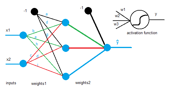
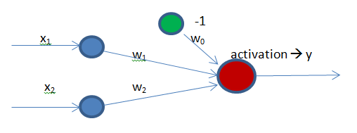
In terms of code, a perceptron is basically a vector of weights which multiplies an input vector and gives an output which is given to a transfer function to determine whether the input belongs to one class or another. Example:

[latex]input = [0.245 \quad 0.942 \quad 0.441] \\
weights = [0.1 \quad 0.32 \quad 0.63 \quad 0.04] \\
sum = -1*0.1 + 0.245*0.1 + 0.942*0.32 + 0.942*0.63 + 0.441*0.04 \\
class = activation(sum) \\[/latex]

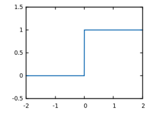
In case of perceptrons, activation function is a simple function which returns 1 if the whole sum is over 0, and return 0 otherwise. This is called step function, because it jumps from 0 to 1 when the input is over 0.

Perceptrons have as many input and output neurons as needed, but they will always have an additional input neuron called bias. The reason why a bias is need is that because without it, the perceptron would not learn about a non-zero input and a zero output or vice versa. When the sum is computed, if all inputs are zero, the result will be therefore zero and the output will inevitably be zero as well. Hence, the weights cannot never learn because the result will always lead to zero.

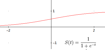
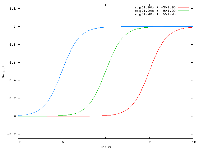
A more mathematical explanation is that despite that the steepness of the activation function can be modified easily without any bias, the bias is responsible for shifting along the X-axis the transfer function. In the following example, we have a one-to-one network and a sigmoid function, however, it can also be explained using the step transfer function described previously.

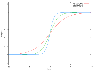
When we have an [latex]x[/latex] dependent argument, the steepness of the sigmoid function can be modified. However, it cannot go anywhere further than 0 when the input is 0. For this, we need a bias.

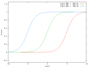
Now, the sigmoid curve can be shifted and we can, for example, get an output of 0 when the input is 2. Usually, the bias has a value of -1 or 1.

As a supervised learning algorithm, perceptron’s learning is based on a training set and a desired output for each input vector, and as a linear classifier, it can classify everything that is linearly separable. Now that we know how the perceptron works, it is time to see how it learns to classify data.

During the learning process, when the classifier receives input data and the classifier is able to classify it correctly, there is no need to make any adjustment. On the contrary, when there is a misclassified input, we need to update and readjust the weights applying the following formula:

[latex]w_i = w_i + \eta (t_i – y_i) x_i \quad[/latex]
(where w = weight, η = learning rate, t = target, y = output, x = input)

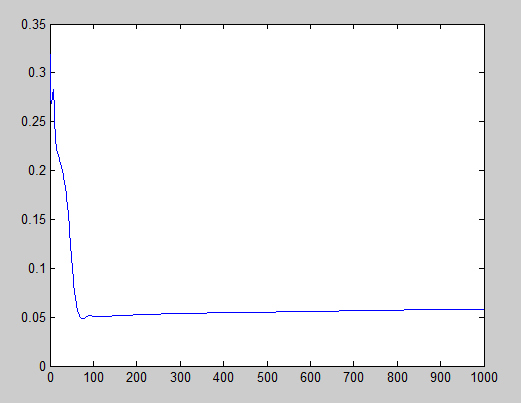
The learning rate plays a key role in perceptrons since it establishes the speed of perceptron’s learning. Before deciding which learning rate is more appropriate, note that a small learning rate may slow down considerably the speed of the learning algorithm and it will need more iterations and consequently more time and resources would be used whereas a big learning rate may make the algorithm jump from the minimum (as we can see in the picture) to climb the mountain that represents the error rate.

Usually, the learning rate is between 0.1 and 0.4 since the weights are small numbers, usually initialized randomly between 0 and 1. Finally, before showing practical examples and Matlab code, it is worth talking about normalization. Normalization it is necessary to keep small weight values which means easy computation. Without normalizing, the algorithm will neither work most of the times. It makes no sense to mix high values (say, values around many thousands) with small values (around 10^-8 values). There is not a unique way to normalize a set of values, but the first one showed me better results.

[latex]y = \frac{x-mean(x)}{var(x)} \\
y = \frac{x-min(x)}{max(x)-min(x)}[/latex]

Example 1: AND

In this case we have a very simple diagram with only two neurons as input and one as output. Additionally, we have a bias connected to the output.

[latex]x_1[/latex]	[latex]x_2[/latex]	[latex]y[/latex]
0	0	0
0	1	0
1	0	0
1	1	1

To solve this problem, we can iterate as many times as needed over our training set until we get no errors.

[latex]\displaystyle\sum_{i=0}^{N} w_i * x_i[/latex]

To learn, we apply the previous learning formula:

[latex]w_i = w_i + \eta (t_i – y_i) x_i[/latex]

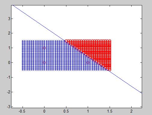
After we finish iterating with no errors, we can build up the decision boundary using this formula:

[latex]y = \frac{-w_1*x + w_0}{w_2} \quad \to \quad w_2*y+w_1*x = w_0[/latex]

All elements at one side of the previous formula belong to a class whereas at the other side they belong to the other class.

AND samples and the decision boundary were drawn. We could be sure about that the result will converge because the different classes are linearly separable (by a plane).

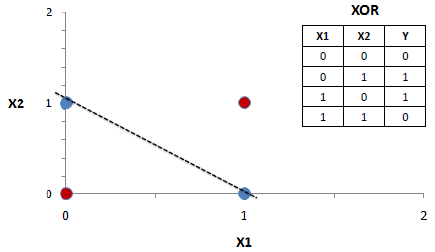
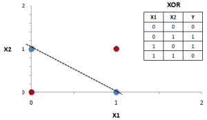
Example 2: XOR

This is the best example to see how Perceptron fails at classifying XOR since it is not possible to separate both classes using only one line, in contrast with other logic functions. If we try to use the perceptron here, it will endlessly try to converge.

This problem can be actually solved by perceptron if we add an additional output neuron. You can think about it trying to imagine this problem in 3 dimensions. In that case, it would be linearly separable.

Example 3: Evolution of the decision boundary

Let us use pseudorandom data:

data = 0.5 + (4-0.5).*rand(66,2);
data = [data ones(66,1)];
data2 = 5 + (10-5).*rand(34,2);
data2 = [data2 zeros(34,1)];
data = [data;data2];

Adding a plot in each iteration:

x = -3:13;
y = (-weights(2)*x+weights(1))/weights(3);
plot(x,y,'m');

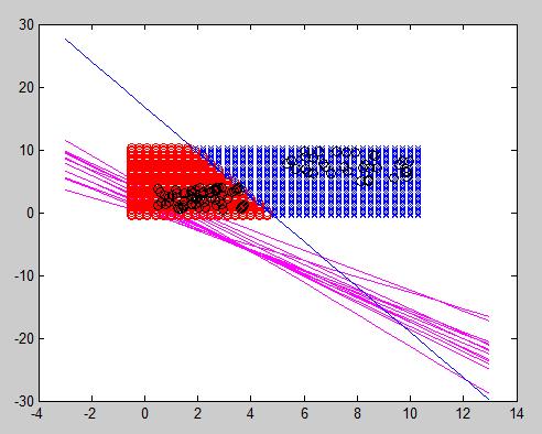
We can see the evolution of the decision boundary:

In this example, we can see that boundaries are not located at the same distance since different amounts of samples have been used. Using the same amount, the distance between the closest elements would be the same.

Example 4: Distinguishing more than 2 classes

A naive attempt to simplify the amount of output neurons would be stating that 2 output neurons can classify up to 4 different classes since [latex]2^N = 4[/latex]. The 00 class would be class A, 01 class B, and so on. Nonetheless, the weights which go from input neurons to a certain output are able to classify just one element, so if 4 different classes are aimed to be distinguished, the same number of output neurons are needed.

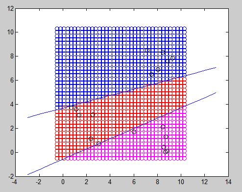
In the figure below, 3 different elements can be properly classified. The 2 output neurons perceptron can only distinguish one feature from another. In this example, 3 classes are differentiated: class B (blue), R and M, which respectively correspond to 01, 00 and 10 output.

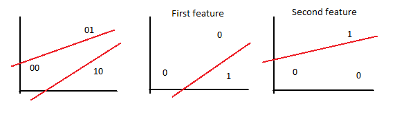
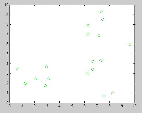
In this particular case, due to the position of each sample, it was possible to draw two straight lines through the whole training data. The next figure represents an example where unfortunately it is not possible to separate one feature from another. 6 samples from each of the 3 classes were chosen. In this case, the algorithm will endlessly try to converge without any valid result. In conclusion, for each feature to be distinguished, an output neuron is needed, but it still needs to be linearly separable.

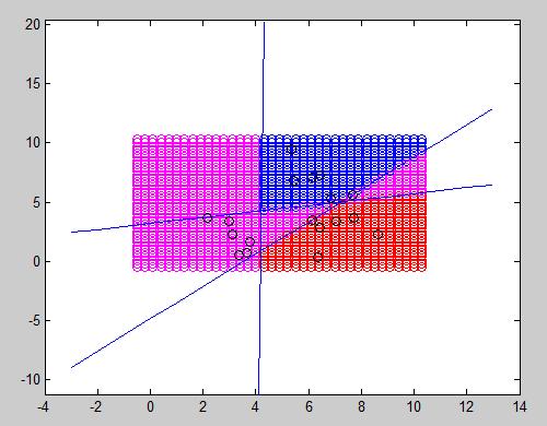
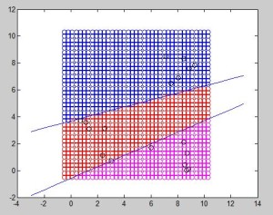
Using as many output neurons as you want is not a panacea. In practice, as we can see below it may work sometimes when a straight line can separate a class from the rest of them (and even in this case, you can see that it has an odd behavior in some magenta regions that need to be specially treated.

Finally, we have a case in which no line can be drawn to separate a class from the rest of them. It will always include a sample from other class. This algorithm definitely works better with few elements in each class because it will be able to linearly separate them, but this does not mean that it does a good work extrapolating new cases (for what the algorithm is suppose to be used).

Conclusions

Despite it seems that perceptrons can perform very poorly, they can be extremely powerful with datasets that undoubtedly are linearly separable since the algorithm is very simple and therefore they can be implemented in very basic systems such as an 8-bit board.

Additionally, perceptrons are academically important since their next evolution, the multilayer perceptron, is fairly used in many types of applications, from recognition/detection systems to control systems.

The code is provided in the Source code section.