History and Evolution
In order to detect edges, it seems obvious that we need to compare the intensity of adjacent pixels (vertical and horizontal). If the difference is high, we will probably have found an edge.
[latex]
E_x = P_{x,y} – P_{x+1,y} \quad \text{vertical} \\
E_y = P_{x,y} – P_{x,y+1} \quad \text{horizontal}
[/latex]
After we combine them:
[latex]
E_{x,y} = P_{x,y} – P_{x+1,y} + P_{x,y} – P_{x,y+1} \\
E_{x,y} = 2*P_{x,y} – P_{x,y+1} – P_{x+1,y}
[/latex]
Therefore, our coefficients are:
[latex]
K = \begin{bmatrix}
2 & -1\\
-1 & 0
\end{bmatrix}
[/latex]
Trough an Taylor series analysis (you can find the formulas in pages 119 and 120 of the referenced book) we can see that by differencing adjacent points we get an estimate of the first derivative at a point with error [latex]O(\Delta x)[/latex] which is the separation between points. This operation reveals that this error can be reduced by spacing the differenced points by one pixel (averaging tends to reduce noise). This is equivalent to computing the first order difference viewed in the previous formula at two adjacent points, as a new difference where:
[latex]
Exx_{x,y} = Ex_{x+1,y} + Ex_{x,y} \\
Exx_{x,y} = P_{x+1,y} – P_{x,y} + P_{x,y} – P_{x-1,y} \\
Exx_{x,y} = P_{x+1,y} – P_{x-1,y}
[/latex]
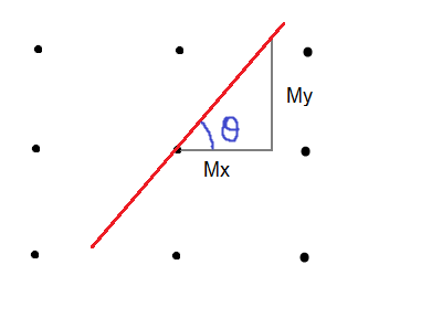
Hence:
[latex]
Mx = \begin{bmatrix}
1 & 0 & -1
\end{bmatrix}
\quad
My = \begin{bmatrix}
1 \\
0 \\
-1
\end{bmatrix}
[/latex]
Prewitt edge detection operator extended both templates by adding two additional rows (or columns). This is due to the fact that averaging reduce noise.
[latex]
Mx = \begin{bmatrix}
1 & 0 & -1 \\
1 & 0 & -1 \\
1 & 0 & -1
\end{bmatrix}
\quad
My = \begin{bmatrix}
1 & 1 & 1 \\
0 & 0 & 0 \\
-1 & -1 & -1
\end{bmatrix}
[/latex]
Finally, we can say that the Sobel edge detector is a simple modification of this.
Application
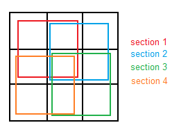
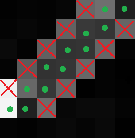
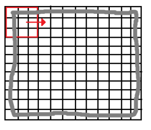
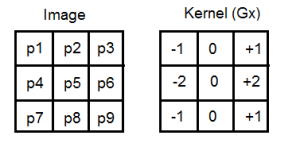
The application of this algorithm is as any other kernel based algorithm. We have two different kernels that need to be applied (convolved) to the image independently. This is done by shifting the kernel through the rows and columns as depicted, and multiplying by each element.
[latex]
G_x = \begin{bmatrix}
-1 & 0 & +1 \\
-2 & 0 & +2 \\
-1 & 0 & +1
\end{bmatrix}
\quad \text{and} \quad
G_y = \begin{bmatrix}
-1 & -2 & -1 \\
0 & 0 & 0 \\
+1 & +2 & +1
\end{bmatrix}
[/latex]
The kernel’s size is odd (typically 3 or 5) so there is no problem fixing it and having a centered valued. During each iteration, we need to multiply each element of the windowed picture with each element of the kernel, and sum it together.
[latex]
V_x = -1*p_1 + 0*p_2 + 1*p_3 + -2*p_4 + 0*p_5 + 2*p_6 -1*p_7 + 0*p_8 + 1*p_9
[/latex]
As I have said previously, during each iteration we need to compute Gx and Gy kernels, so we will end up with two values. The following operation is needed, and its result will be placed in the position of middle of the matrix (P5) in a different matrix which will have the final image:
[latex]
G = \sqrt{G_x^2 + G_y^2}
[/latex]
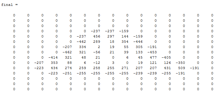
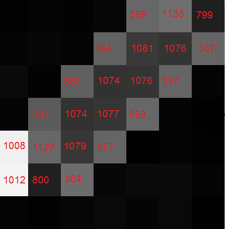
Note that because of this procedure, borders (2 images below marked with gray) will be lost. The larger is the kernel’s size, the more border will be lost. Nonetheless, this is not usually a problem since our goal is usually located at the center of the image.
In conclusion, the algorithm may be the following:
Iterate over rows
Iterate over columns
Convolve the windowed region with Gx
Convolve the windowed region with Gy
Solve square root
Write that value on the output picture
About Sobel templates
[latex]
G_x = \begin{bmatrix}
-1 & 0 & +1 \\
-2 & 0 & +2 \\
-1 & 0 & +1
\end{bmatrix}
\quad \text{and} \quad
G_y = \begin{bmatrix}
-1 & -2 & -1 \\
0 & 0 & 0 \\
+1 & +2 & +1
\end{bmatrix}
[/latex]
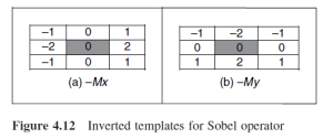
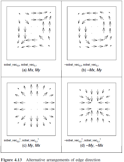
These templates are probably the most used that you can find in the literature about Sobel filter, but you can actually see that when using Sobel filter in Canny edge detector I used a slightly different ones.
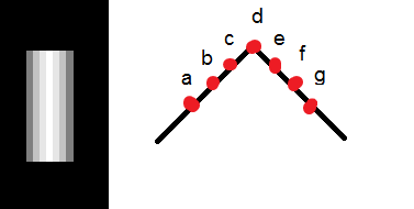
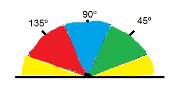
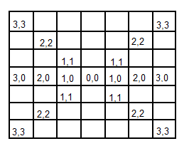
This is because Sobel edge direction data can be arranged in different ways without modifying the general idea of the filter. Therefore, depending on the template’s orientation, points will have different directions, as we can see in the following pictures extracted from the book I used.
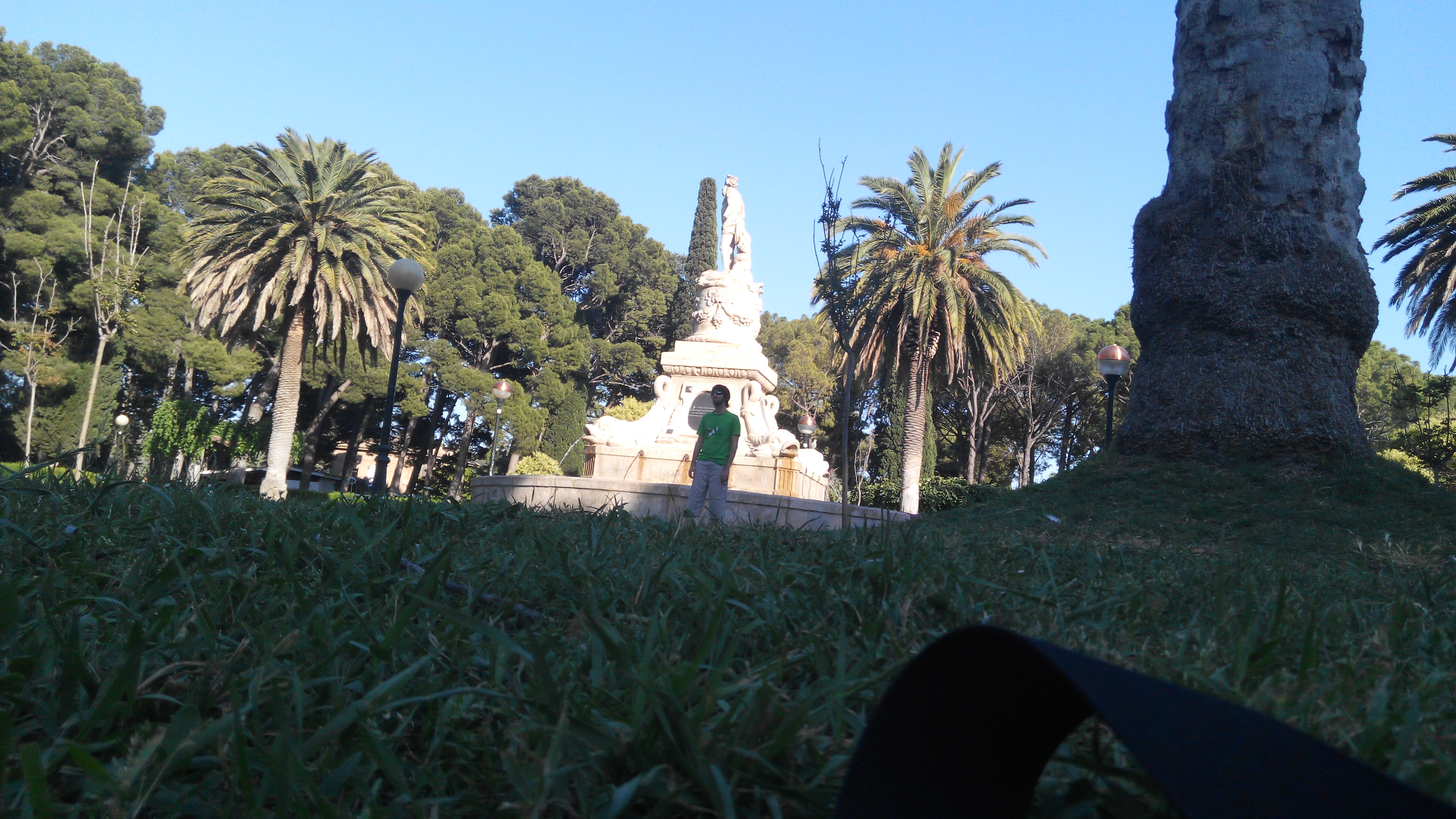
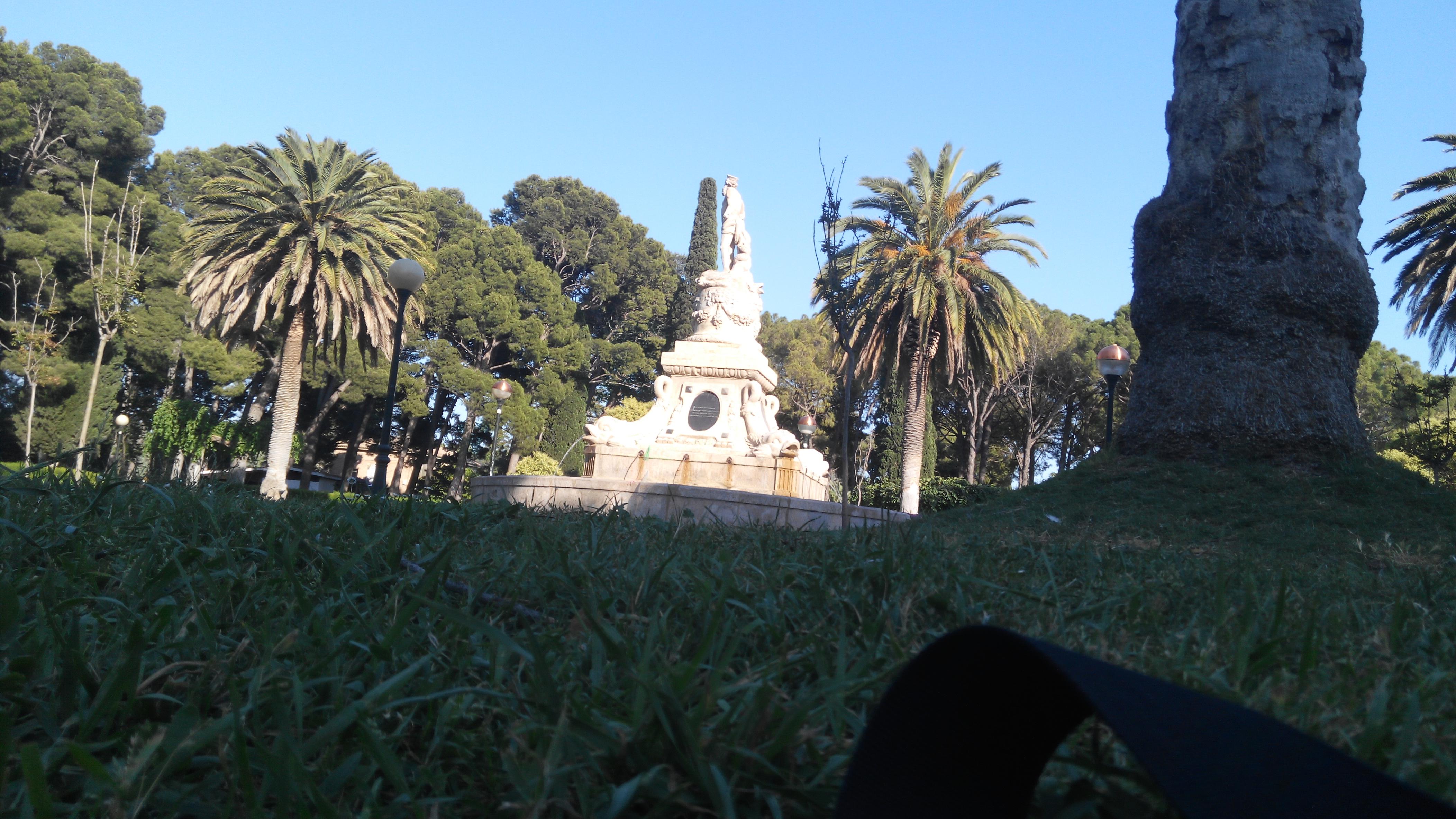
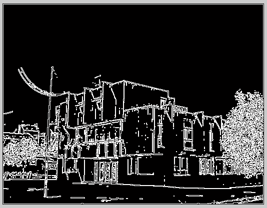
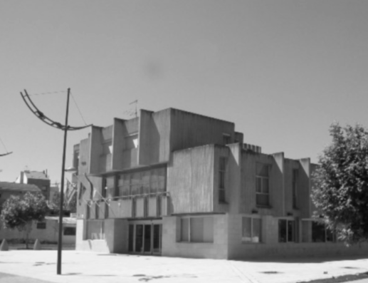
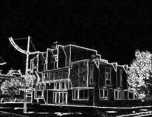
Results
 |
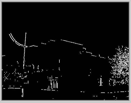
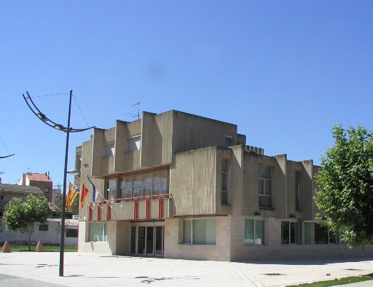
| Original |
|
|
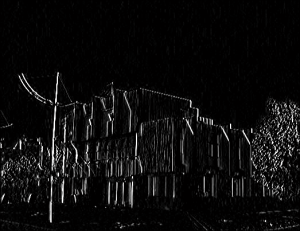 |
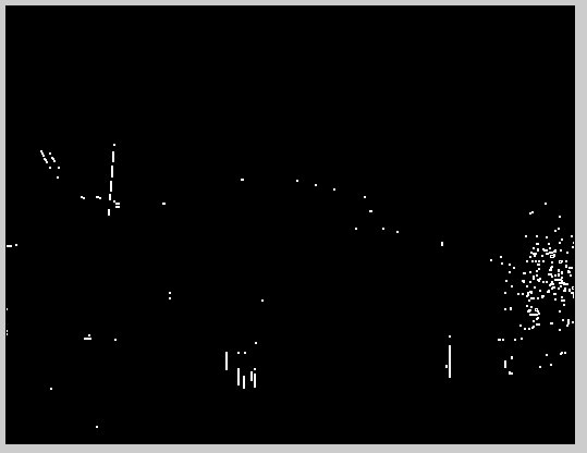
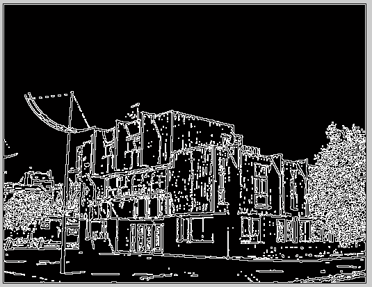
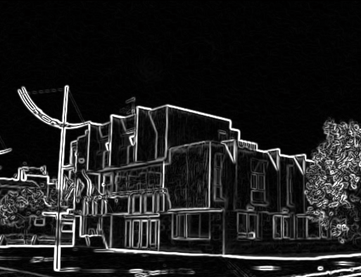
| Sobel Y-axis |
|
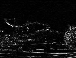 |
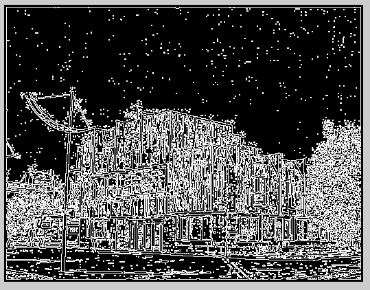
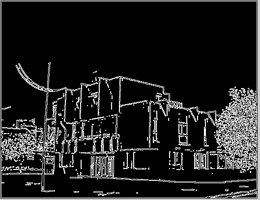
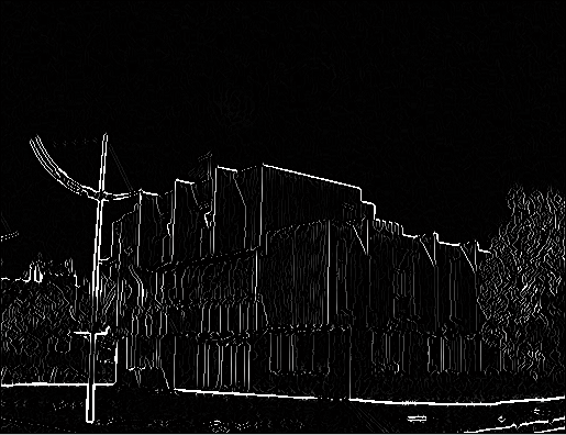
| Sobel X-axis |
|
|
 |
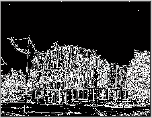
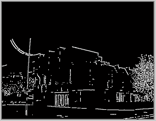
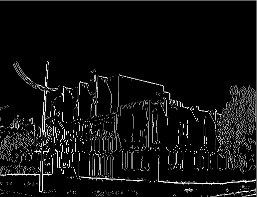
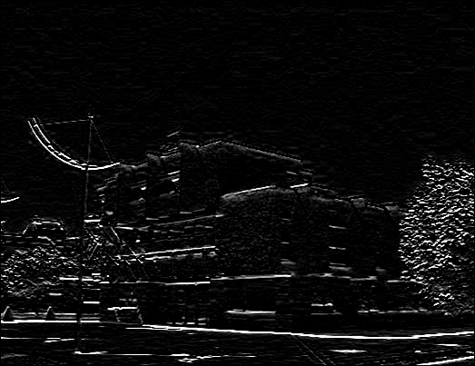
| Sobel (combined) |
|
The code is provided in the Source code section.
References
1. M. Nixon and A. Aguado. 2008. “First order edge detection operators”, Feature Extraction & Image Processing.