Sigmoid and its main problem
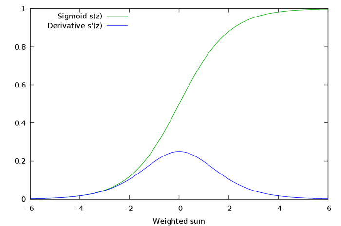
Sigmoid function has been the activation function par excellence in neural networks, however, it presents a serious disadvantage called vanishing gradient problem. Sigmoid function’s values are within the following range [0,1], and due to its nature, small and large values passed through the sigmoid function will become values close to zero and one respectively. This means that its gradient will be close to zero and learning will be slow.
This can be easily seen in the backpropagation algorithm (for a simple explanation of backpropagation I recommend you to watch this video):
[latex]-(y-\hat{y}) f’ (z) \frac{\partial z}{\partial W}[/latex]
where [latex]y[/latex] is the prediction, [latex]\hat{y}[/latex] the ground truth, [latex]f'()[/latex] derivative of the sigmoid function, [latex]z[/latex] activity of the synapses and [latex]W[/latex] the weights.
The first part [latex]-(y-\hat{y}) f’ (z)[/latex] is called backpropagation error and it simply multiplies the difference between our prediction and the ground truth times the derivative of the sigmoid on the activity values. The second part describes the activity of each synopsis. In other words, when this activity is comparatively larger in a synapse, it has to be updated more severely by the previous backpropagation error. When a neuron is saturated (one of the bounds of the activation function is reached due to small or large values), the backpropagation error will be small as the gradient of the sigmoid function, resulting in small values and slow learning per se. Slow learning is one of the things we really want to avoid in Deep Learning since it already will consist in expensive and tedious computations. The Figure below shows how the derivative of the sigmoid function is very small with small and large values.

Conclusion: if after several layers we end up with a large value, the backpropagated error will be very small due to the close-to-zero gradient of the sigmoid’s derivative function.
ReLU activation function
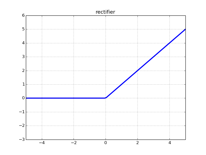
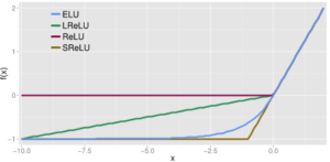
ReLU (Rectified Linear Unit) activation function became a popular choice in deep learning and even nowadays provides outstanding results. It came to solve the vanishing gradient problem mentioned before. The function is depicted in the Figure below.

The function and its derivative:
latex
f(x) = \left \{ \begin{array}{rcl}
0 & \mbox{for} & x < 0\\
x & \mbox{for} & x \ge 0\end{array} \right.
latex
latex
f'(x) = \left \{ \begin{array}{rcl}
0 & \mbox{for} & x < 0\\
1 & \mbox{for} & x \ge 0\end{array} \right.
/latex
In order to understand why using ReLU, which can be reformulated as [latex]f(x) = max(0,x)[/latex], is a good idea let's divide the explanation in two parts based on its domain: 1) [-∞,0] and 2) (0,∞].
1) When the synapse activity is zero it makes sense that the derivative of the activation function is zero because there is no need to update as the synapse was not used. Furthermore, if the value is lower than zero, the resulting derivative will be also zero leading to a disconnection of the neuron (no update). This is a good idea since disconnecting some neurons may reduce overfitting (as co-dependence is reduced), however this will hinder the neural network to learn in some cases and, in fact, the following activation functions will change this part. This is also refer as zero-sparsity: a sparse network has neurons with few connections.
2) As long as values are above zero, regardless of how large it is, the gradient of the activation function will be 1, meaning that it can learn anyways. This solves the vanishing gradient problem present in the sigmoid activation function (at least in this part of the function).
Some literature about ReLU [1].
LReLU activation function
Leaky ReLU is a modification of ReLU which replaces the zero part of the domain in [-∞,0] by a low slope, as we can see in the figure and formula below.
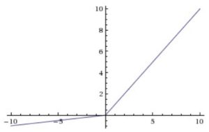
The function and its derivative:
latex
f(x) = \left \{ \begin{array}{rcl}
0.01 x & \mbox{for} & x < 0\\
x & \mbox{for} & x \ge 0\end{array} \right.
latex
latex
f'(x) = \left \{ \begin{array}{rcl}
0.01 & \mbox{for} & x < 0\\
1 & \mbox{for} & x \ge 0\end{array} \right.
latex
The motivation for using LReLU instead of ReLU is that constant zero gradients can also result in slow learning, as when a saturated neuron uses a sigmoid activation function. Furthermore, some of them may not even activate. This sacrifice of the zero-sparsity, according to the authors, can provide worse results than when the neurons are completely deactivated (ReLU) [2]. In fact, the authors report the same or insignificantly better results when using PReLU instead of ReLU.
PReLU activation function
Parametric ReLU [3] is a inspired by LReLU wich, as mentioned before, has negligible impact on accuracy compared to ReLU. Based on the same ideas that LReLU, PReLU has the same goals: increase the learning speed by not deactivating some neurons. In contrast with LReLU, PReLU substitutes the value 0.01 by a parameter [latex]a_i[/latex] where [latex]i[/latex] refers to different channels. One could also share the same values for every channel.
The function and its derivative:
latex
f(x) = \left \{ \begin{array}{rcl}
a_i x & \mbox{for} & x < 0\\
x & \mbox{for} & x \ge 0\end{array} \right.
latex
latex
f'(x) = \left \{ \begin{array}{rcl}
a_i & \mbox{for} & x < 0\\
1 & \mbox{for} & x \ge 0\end{array} \right.
latex
The following equation shows how these parameters are iteratevely updated using the chain rule as the weights in the neural network (backpropagation). [latex]\mu[/latex] is the momentum and [latex]\epsilon[/latex] is the learning rate. IN the original paper, the initial [latex]a_i[/latex] used is 0.25
[latex]\nabla a_i := \mu \nabla a_i + \epsilon \frac{\partial \varepsilon}{\partial a_i}[/latex]
RReLU activation function
Randomized ReLU was published in a paper [4] that compares its performance with the previous rectified activations. According to the authors, RReLU outperforms the others, and LReLU performs better when [latex]\frac{1}{5.5}[/latex] substitutes 0.01.
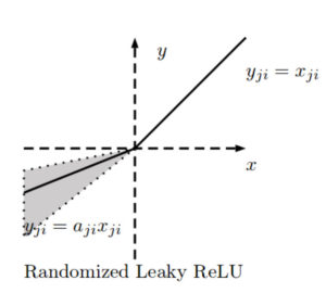
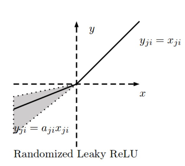
The negative slope of RReLU is randomly calculated in each training iteration such that:
[latex]f_{ji}(x) = \left \{ \begin{array}{rcl} \frac{x_{ji}}{a_{ji}} xa & \mbox{for} & x_{ji} \ge 0\\ x_{ji} & \mbox{for} & x_{ji} \ge 0\end{array} \right.[/latex]
where
[latex]a_{ji} \sim U(l,u)[/latex]
The motivation to introduce a random negative slope is to reduce overfitting.
[latex]a_{ji}[/latex] is thus a random number from a uniform distribution bounded by [latex]l[/latex] and [latex]u[/latex] where [latex]i[/latex] refers to the channel and [latex]j[/latex] refers to the example. During the testing phase, [latex]a_{ji}[/latex] is fixed, and an average of all the [latex]a_{ji}[/latex] is taken: [latex]a_{ji} = \frac{l+u}{2}[/latex]. In the paper they use [latex]U(3,8)[/latex] and in the test time [latex]a_{ji} = \frac{11}{2}[/latex].
ELU activation function
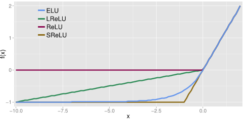
Exponential Linear Unit (ELU) is another type of activation function based on ReLU [5]. As other rectified units, it speeds up learning and alleviates the vanishing gradient problem.
Similarly to the previous activation functions, its positive part has a constant gradient of one so it enables learning and does not saturate a neuron on that side of the function. LReLU, PReLU and RReLU do not ensure noise-robust deactivation since their negative part also consists on a slope, unlike the original ReLU or ELU which saturate in their negative part of the domain. As explained before, saturation means that the small derivative of the function decreases the information propagated to the next layer.
The activations that are close to zero have a gradient similar to the natural gradient since the shape of the function is smooth, thus activating faster learning than when the neuron is deactivated (ReLU) or has non-smooth slope (LReLU).
The function and its derivative:
[latex]f(x) = \left \{ \begin{array}{rcl} \alpha (exp(x) – 1) & \mbox{for} & x \le 0\\ x & \mbox{for} & x > 0\end{array} \right.[/latex]
[latex]f'(x) = \left \{ \begin{array}{rcl} f(x) + \alpha & \mbox{for} & x \le 0\\ 1 & \mbox{for} & x > 0\end{array} \right.[/latex]
In a nutshell:
- Gradient of 1 in its positive part.
- Deactivation on most of its negative domain.
- Close-to-natural gradient in values closer to zero.
Softmax activation function
For the sake of completeness, let’s talk about softmax, although it is a different type of activation function.
Softmax it is commonly used as an activation function in the last layer of a neural network to transform the results into probabilities. Since there is a lot out there written about softmax, I want to give an intuitive and non-mathematical reasoning.
Case 1:
Imagine your task is to classify some input and there are 3 possible classes. Out of the neural network you get the following values (which are not probabilities): [3,0.7,0.5].
It seems that it’s very likely that the input will belong to the first class because the first number is clearly larger than the others. But how likely is it? We can use softmax for this, and we would get the following values: [0.846, 0.085, 0.069].
Case 2:
Now we have the values [1.2,1,1.5]. The last class has a larger value but this time is not that certain whether the input will belong to that class but we would probably bet for it, and this is clearly represented by the output of the softmax function: [0.316, 0.258, 0.426].
Case 3::
Now we have 10 classes and the values for each class are 1.2 except for the first class which is 1.5: [1.5,1.2,1.2,1.2,1.2,1.2,1.2,1.2,1.2,1.2]. Common sense says that even if the first class has a larger value, this time the model is very uncertain about its prediction since there are a lot of values close to the largest one. Softmax transforms that vector into the following probabilities: [0.13, 0.097, 0.097, 0.097, 0.097, 0.097, 0.097, 0.097, 0.097, 0.097].
Softmax function:
[latex size=”25″]\sigma (z)_j = \frac{e^{z_j}}{\sum^K_{k=1} e^{z_j}}[/latex]
In python:
z_exp = [math.exp(i) for i in z]
sum_z_exp = sum(z_exp)
return [round(i/sum_z_exp, 3) for i in z_exp]
References
1. Nair V. & Hinton G.E. 2010. “Rectified Linear Units Improve Restricted Boltzmann Machines”
2. Maas A., Hannun A.Y & Ng A.Y. 2013. “Rectifier Nonlinearities Improve Neural Network Acoustic Models”
3. He K., Zhang X., Ren S. & Sun J. 2015. “Delving Deep Into Rectifiers: Surpassing Human-Level Performance on ImageNet Classification”
4. Xu B., Wang N., Chen T. & Li M. 2015. “Empirical Evaluation of Rectified Activations in Convolutional Network”
5. Clevert D.A., Unterthiner T. & Hochreiter S. 2016. Fast and Accurate Deep Network Learning by Exponential Linear Units (ELUs)